


1 Introduction
Graphene in an isolated state has been explored in 2004 and since then it has procured attention of researchers all over the globe due to its exceptional properties. It is tested to be the hardest and thinnest nanoscale material consisting of a single layer of carbon atoms arranged in hexagonal filigree. Since all the atoms in graphene are surface atoms, therefore, it is quite responsive to mechanical, thermal, optical, and electronic effects,[1-7] which make it a key candidate for industrial applications.[8-11] Moreover, Quantum Hall effects are observed for graphene at moderate temperature.[12]
Wrinkles have been observed in graphene sheets caused by scanning tunneling microscopy (STM) of graphene topographs on Si${\rm O}_2$ in Ref. [13]. Properties like electric conductivity and quantum transport are significantly affected by these wrinkle channels.[14-15] Wrinkles have been proved to be a good prospect in designing flexible electric sensors[16] and to assemble graphene nanoribbons.[17] Apart from these mentioned contributions, there are a lot of unaddressed issues like the absence of theoretical model depicting the formation process and the lack of knowledge to analyze the propagation properties of wrinkles.[18]
The well known KdV equation interprets the motion of single-soliton reads as
$ \%\label{kdv} \frac{\partial u}{\partial t}+u\frac{\partial u}{\partial x}+\frac{\partial^3 u}{\partial x^3}=0. $
Solution of Eq. (1) is $u = 3vh^2(\sqrt{v}/2 )(x - vt)$, where $v$ portrays the velocity profile of soliton. The thermophoretic motion (TM) and shape of wrinkles in graphene are very akin to the solitary wave in its properties. In correspondence with Ref. [19], the structural shape of wrinkle at different positions derived through MD simulation by fitting a quadratic polynomial has the form: $u_w=3 c_w\,h^2\left((\sqrt{c_w}/2)[x-at^2/2-bt]\times c_w\right)$, where $a$ and $b$ are constants, and $c_w$ can be tailored to make $u_w$ consistent with the shape of the wrinkle. The motion equation satisfied by $u_w$ is given by
$ \%\label{tkdv} \frac{\partial u_w}{\partial t}+u_w\frac{\partial u_w}{\partial x}+\frac{\partial^3 u_w}{\partial x^3}+(a t+b-c_w)\frac{\partial u_w}{\partial x}=0. $
The wrinkle motion is in accordance with that of single-soliton as it remains unaffected during its course of motion. In a comparison of Eq. (2) with KdV equation, the additional term $(a t + b - c_w) (\partial u_w/\partial x)$ represents the driving force captured through thermal gradients and is held responsible for the acceleration of wrinkles.
A number of techniques have been developed to study the integrability and to construct multiple-solitary wave solutions of nonlinear partial differential equations including inverse scattering,[22-24] Hirota's bilinear method and its simplified form.[25-30] In Refs. [29-30], Eq. (2) was investigated to study the wave propagation of the N-soliton solutions. These solutions have been derived via Hirota's bilinear method with the aid of symbolic computations. Furthermore, the shape, amplitude, open direction and width of the N-solitons are controllable through certain parameters.
The theme of this paper is to use the generalized unified method,[31-33] which is the generalization of the simple unified method presented in Refs. [34-37]. The paper is categorized in three sections. Section 2 is devoted to the study of multi-soliton solution of the TM equation along with their graphics using the GUM. We will conclude our paper in Sec. 3.
2 Multi-soliton Solutions of TM Equation by GUM
$ \label{eqw} \Omega_t+\Omega_{xxx}+\frac{\Omega^2_x}{2}+(a t+b-c_w)\Omega_x=0. $
$ \label{eq7} \Omega(x,t)=\Gamma(\xi_1)=\frac{p_0+p_1\psi_1(\xi_1)}{q_0+q_1\psi_1(\xi_1)}, $
where $\xi_1=\alpha_1x+\int\alpha_2(t) {\rm d}t$. Here $p_0,p_1,q_0$ and $q_1$ are unknowns to be determined. By inserting Eq. (4) into Eq. (3) and equating the coefficients of $\psi_i(\xi_i)$ to zero gives a system of algebraic equations whose solution is given by
$ q_0 =q_1=1,~~~p_{{1}}= ( 12\,c_{1}\alpha_{{1}}+ p_0), \\ \alpha_{{2}}(t)=-\alpha_{{1}}(c_{1}^{2}\alpha_{1}^{2}-c_{{w}}+b+at)\,. $
Using Eq. (5) along with auxiliary function $\psi_1(\xi_1)$ in Eq. (4), we get
$ \Omega(x,t)=\Gamma(\xi_1)=\frac{p_0+ \left( 12\,c_{{1}}\alpha_{{1}}+ p_0\right){\rm e}^{c_1\xi_1}}{1+{\rm e}^{c_1\xi_1}}. $
As $u(x,t)=\Omega_x(x,t)$, so we have
$ \label{eq9} u=3c_1^2\alpha_1^2h^2\left(\frac{c_1\xi_1}{2}\right). $
It is quite evident that the one-soliton solution in Eq. (7) can be compared to that reported in Ref. [19] for
$c_w=c_1^2\alpha_1^2$.
2.2 2-soliton Solutions of TM Equation
$ \%\label{s2} \Omega(x,t) = \Gamma(\xi_1,\xi_2) \\ =\frac{p_0+p_1\psi_1(\xi_1)+p_2\psi_2(\xi_2)+p_3\psi_1(\xi_1) \psi_2(\xi_2)}{q_0+q_1\psi_1(\xi_1)+q_2\psi_2(\xi_2)+q_3\psi_1(\xi_1) \psi_2(\xi_2)}, $
where $\xi_1 = \alpha_1x+\int\alpha_2(t) {\rm d}t, \xi_2 = \beta_1x+\int\beta_2(t){\rm d}t$ and $p_i$ and $q_i$ are arbitrary parameters to be evaluated, $i=0,1,2$. The functions $\psi_i(\xi_i)$ are obtained from the first order differential equations $\psi_1^{\prime}(\xi_1) = b_1\psi_1(\xi_1)$ and $\psi_2^{\prime}(\xi_2) = c_1\psi_2(\xi_2)$. By plugging Eq. (8) into Eq. (3) and by equating the coefficients of $\psi_i(\xi_i)$ to zero, we get a system of algebraic equations whose solution is given by
\begin{eqnarray}\label{solution_2}\nonumber p_0&=&-12\alpha_1b_1q_0+\frac{S^2_{-}p_1q_2}{S^2_{+}q_3}\,,\quad p_2=\frac{q_2\left(S^2_{-}p_1q_2/S^2_{+}q_3-12q_0S_{-}\right)}{q_0}\,,\quad p_3=\frac{q_2S^2_{-}\left(p_1+12\beta_1c_1q_3q_0S^2_{+}/q_2S^2_{-}\right)}{q_0S^2_{+}},\\\nonumber q_1&=&\frac{q_3q_0S^2_{+}}{q_2S^2_{-}}\,,\quad \alpha_2(t)=-\alpha_1(a t+b+b^2_1\alpha^2_1-c_w)\,,\quad \beta_2(t)=-\beta_1(a t+b+c^2_1\beta^2_1-c_w), \end{eqnarray}
where $S_{\pm}=\alpha_1b_1\pm\beta_1c_1$.
By utilizing the above solution into Eq. (8), we get the solution of Eq. (2) namely,
$ u(x,t)=\dfrac{12e^{b_1\xi_1}(b^2_1\alpha_1^2q_0+c_1^2\beta_1^2 q_3e^{b_1\xi_1+c_1\xi_2})(q_0q_3S^2_{+}/q_{2}S^2_{-})+12 e^{c_1\xi_2}(c^2_1\beta_1^2q_2q_0+b_1^2\alpha_1^2q_2q_3 e^{b_1\xi_1+c_1\xi_2}+2q_3q_0S^2_{+}e^{b_1\xi_1})} {(q_0+(q_3q_0S^2_{+}/q_2S^2_{-})\,e^{b_1\xi_1}+q_2\,e^{c_1\xi_2}+ q_3\,e^{b_1\xi_1+c_1\xi_2})^2}, $
where $\xi_1=\alpha_1x-\alpha_1(a t/2+b+b^2_1\alpha^2_1-c_w)t,~\xi_2=\beta_1x-\beta_1(at/2+b+c^2_1\beta^2_1-c_w)t.$ The solution is depicted graphically in Fig. 1 for different values of the parameters.
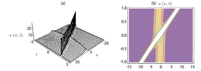
Fig. 1 Evolution of two solitons: (a) 3D-plot (b) The projection view of (a), for $c_1=1/2,~b_1=3,~q_2=1/5,~q_0=1/20,~c_w=1/10,~p_1=3/20,~\alpha_1=1,~\beta_1=2,~a=0.3,~b=-0.5,~q_3=1$. |
$ u(x,t)=\Omega_x(x,t)\,,\\ \Omega(x,t)=\Gamma(\xi_1,\xi_2,\xi_3)=\frac{p_0+\sum^3_{i=1} p_i\psi_i(\xi_i)+\sum^3_{i,j=1}p_{ij}\psi_i(\xi_i)\psi_j(\xi_j)+ p_{123}\psi_1(\xi_1)\psi_2(\xi_2)\psi_3(\xi_3)} {q_0+\sum^3_{i=i}q_i\psi_i(\xi_i)+\sum^3_{i,j=1}q_{ij}\psi_i (\xi_i)\psi_j(\xi_j)+q_{123}\psi_1(\xi_1)\psi_2(\xi_2)\psi_3(\xi_3)}, $
where $i < j$ and $\xi_1=\alpha_1x+\int\alpha_2(t) {\rm d}t,~\xi_2=\beta_1x+\int\beta_2(t){\rm d}t, ~\xi_3=\gamma_1x+\int\gamma_2(t) {\rm d}t$ and $p_i,~p_{ij},~p_{123}$ as well as $q_i,~q_{ij},~q_{123}$ are arbitrary constants to be evaluated, while $i,j=1,2,3$. The auxiliary functions $\psi_i(\xi_i)$ satisfy $\psi_1^{\prime}(\xi_1) = b_1\psi_1(\xi_1)$, $\psi_2^{\prime}(\xi_2) = c_1\psi_2(\xi_2)$, and $\psi_3^{\prime}(\xi_3) = s_1\psi_3(\xi_3)$. By plugging Eq. (10) into Eq. (3) and by equating the coefficients of $\psi_i(\xi_i)$ and $\psi_i(\xi_i)\psi_j(\xi_j)$ to zero, we get a system of algebraic equations whose solution is given by
$$ p_0 = \frac{1}{H^2_{+}R^2_{+}q_{123}}[-12b^5_1\alpha^5_1q_0q_{123}+c^2_1\beta^2_1p_1q_{23}\gamma^2_1s^2_1 +b^4_1\alpha^4_1(p_1q_{23}-24q_{123}q_0T_{+}) +b^2_1\alpha^2_1(p_1q_{23}\gamma^2_1s^2_1+c^2_1\beta^2_1(p_1q_{23}-24q_{123}q_0\gamma_1s_1) \\ +4c_1\beta_1\gamma_1s_1(p_1q_{23}-6q_{123}q_0\gamma_1s_1)) -2b_1c_1\alpha_1\beta_1\gamma_1s_1(p_1q_{23}\gamma_1s_1+c_1\beta_1 (p_1q_{23}+6q_{123}q_0\gamma_1s_1))-2b^3_1\alpha^3_1(6c_1^2\beta_1^2q_{123}q_0 \\ +\gamma_1s_1(p_1q_{23}+6q_{123}q_0\gamma_1s_1)+c_1\beta_1 (p_1q_{23}+24q_{123}q_0\gamma_1s_1))], \\ p_2 =-\frac{1}{H^2_{+}T^2_{+}R^2_{+}q_{123}q_3}[q_{23}H_{-}T^2_{+} (12b_1^4\alpha_1^4q_{123}q_0+c_1\beta_1(p_1q _{23}+12c_1\beta_1q_{123}q_0))\gamma_1^2s_1^2 +b_1\alpha_1\gamma_1s_1(-2c_1\beta_1p_1q_{23}+24c_1^2 \beta_1^2q_{123}q_0 \\ -p_1q_{23}\gamma_1s_1+24c_1\beta_1q_{123}q_0\gamma_1s_1) +b_1^3\alpha_1^3(-p_1q_{23}+24q_{123}q_0T_{+}) +b_1^2\alpha_1^2(12c_1^2\beta_1^2q_{123}q_0+2\gamma_1s_1(p_1q_{23} +6q_{123}q_0\gamma_1s_1) \\ +c_1\beta_1(p_1q_{23}+48q_{123}q_0\gamma_1s_1))]\,, \\ p_3=-\frac{q_3R_{-}}{H^2_{+}R^2_{+}q_{123}q_0}[12b_1^4\alpha_1^4q_{123}q_0+c_1^2\beta_1^2\gamma_1s_1 (p_1q_{23}+12q_{123}q_0\gamma_1s_1)+b_1^3\alpha_1^3(-p_1q_{23}+24q_{123}q_0T_{+}) +b_1c_1\alpha_1\beta_1(2\gamma_1s_1(-p_1q_{23} \\ +12q_{123}q_0\gamma_1s_1)+c_1\beta_1(-p_1q_{23}+24q_{123}q_0\gamma_1s_1)) +b_1\alpha_1^2(12c_1^2\beta_1^2q_{123}q_0 \\ +\gamma_1s_1(p_1q_{23}+12q_{123}q_0\gamma_1s_1)+2c_1\beta_1(p_1q_{23} +24q_{123}q_0\gamma_1s_1))]\,, \\ p_{12}=\frac{H^2_{-}T^2_{+}q_{23}(p_1+12c_1\beta_1 (H^2_{+}R^2_{+}q_0q_{123})/H^2_{-}R^2_{-}q_{23})}{H^2_{+}T^2_{-}q_{3}}\,, \\ p_{13}=\frac{q_3R^2_{-}(p_1+12H^2_{+}R^2_{+}q_0q_{123}\gamma_1s_1/H^2_{-}R^2_{-}q_{23})}{q_0R^2_{+}}\,, \\ p_{23}=\frac{q_{23}}{H^2_{+}R^2_{+}q_0q_{123}}\bigl[-12b_1^5\alpha_1^5q_0q_{123}+b_1^4 \alpha_1^4(p_1q_{23}-12q_{123}q_0T_{+})+c_1^2\beta_1^2\gamma_1^2s_1^2(p_1q_{23}+12q_{123}q_0T_{+}) +2b_1^3\alpha_1^3(-c_1\beta_1p_1q_{23} \\ +6c_1^2\beta_1^2q_{123}q_0+\gamma_1s_1(-p_1q_{23} +6q_{123}q_0\gamma_1s_1)) +2b_1c_1\alpha_1\beta_1\gamma_1s_1(12c_1^2\beta_1^2q_{123}q_0 +\gamma_1s_1(-p_1q_{23}+12q_{123}q_0\gamma_1s_1) \\ +c_1\beta_1(-p_1q_{23}+18q_{123}q_0\gamma_1s_1))+b_1^2\alpha_1^2(12c_1^3\beta_1^3q_{123}q_0 +4c_1\beta_1\gamma_1s_1(p_1q_{23}+9q_{123}q_0\gamma_1s_1) +\gamma_1^2s_1^2(p_1q_{23}+12q_{123}q_0\gamma_1s_1) \\ +c_1^2\beta_1^2(p_1q_{23}+36q_{123}q_0\gamma_1s_1))\bigr]\,, \\ p_{123}=\frac{1}{H^2_{+}R^2_{+}q_0}[2b_1^3\alpha_1^3T_{+}(-p_1q_{23}+12q_{123}q_0T_{+}) +2b_1c_1\alpha_1\beta_1\gamma_1s_1T_{+}(-p_1q_{23}+12q_{123}q_0T_{+}) b_1^4\alpha_1^4(p_1q_{23}+12q_{123}q_0T_{+}) \\ +c_1^2\beta_1^2\gamma_1^2s_1^2(p_1q_{23}+12q_{123}q_0T_{+}) +b_1^2\alpha_1^2(c_1^2\beta_1^2+4c_1\beta_1\gamma_1s_1+\gamma_1^2s_1^2) (-p_1q_{23}+12q_{123}q_0T_{+})]\,, \\ q_1=\frac{H^2_{+}R^2_{+}q_0q_{123}}{H^2_{-}R^2_{-}q_{23}}\,,\quad\quad q_2 =\frac{T^2_{+}q_0q_{23}}{T^2_{-}}\,,\quad\quad q_{13}=\frac{H^2_{+}q_3q_{123}}{H^2_{-}}\,, \quad\quad q_{12}=\frac{q_{123}q_0R^2_{+}T^2_{+}}{q_3R^2_{-}T^2_{-}}\,, \\ \alpha_2(t)=-\alpha_1(a t+b+b_1^2\alpha_1^2-c_w)\,,\quad\quad \beta_2(t)=-\beta_1(a t+b+c_1^2\beta_1^2-c_w)\,,\quad\quad \gamma_2(t)=-\gamma_1(a t+b+r_1^2s_1^2-c_w)\,, $$
where $H_{\pm}=b_1\alpha_1\pm c_1\beta_1,~R_{\pm}=b_1\alpha_1\pm \gamma_1s_1,~T_{\pm}=c_1\beta_1\pm \gamma_1s_1.$
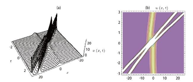
Extracting $\psi_i(\xi_i)$ from $\psi^{\prime}_i(\xi_i)=c_i\psi_i(\xi_i)$ and putting them into Eq. (10) along with the values of the parameters, we get the solution of Eq. (2) which is not written here because of its huge volume. The solution is depicted graphically in Fig. 2 for different values of the parameters.
Fig. 2 Evolution of three solitons: (a) 3D-plot (b) The projection view of (a), for $c_1=1/2,~b_1=3,~s_{1}=0.9~q_{123}=1/5,~q_0=1/20,~c_w=1/10,~p_1=3/20,~\alpha_1=-1, ~\beta_1=2,~\gamma_1=3,~a=0.3,~b=-0.5,~q_3=1,~q_{23}=1$. |
3 Conclusion
This paper investigates the multi-soliton solutions for TM equation, which describes the thermophoresis of wrinkles in graphene sheets. The versatile integration tools, the GUM, is applied to extract 2- and 3-soliton solutions. These solutions are analyzed graphically and it is observed that the width, amplitude, shape and open direction depends on certain parameters. In physical experiments, the single soliton serves as an analogue to simulate the propagation for single wrinkle wave.[19] Therefore, multi-solitons can provide a valuable insight to understand the dynamics of multiple wrinkle waves in graphene nanoribbons. Comparing with the results in Refs. [29-30], we found that: in our paper the obtained solutions had different wave structures and the interaction between these solutions represents an elastic collision. The solutions can be critical to understand attributes of the TM equation through the wonder nano-material graphene sheet.
Compliance with Ethical Standards
Conflict of interests: The authors declare that they have no conflict of interests.