


1 Introduction
Based on Einstein's local realism and hidden variable model, Bell proposed the famous Bell inequality,[1] which is an important resource in the quantum information theory. Chain inequality is an important kind of Bell inequality, which has $n$ ($n\geq2$) measurement bases, and the Clauser-Horne-Shimony-Holt (universally known as CHSH inequality[2]) inequality can be assumed to be a special Chain inequality with $n=2$. More precisely, Chain inequality can be applied to propose device independent quantum information protocols,[3-4] where security of the protocols can be guaranteed by the Chain inequality violation, not based on the perfect quantum states preparation and measurement assumption. More recently, Colbeck et al.[5-10] have proved that the imperfect randomness could be amplified via Chain inequality.
The Bell inequality violation is usually based on the entanglement states preparation and the projective measurement assumption, which will lead to the states collapse after the projective measurement. However, by applying the weak measurement technology, an observer can extract less information about a system with the smaller disturbance.[11-12] The weak measurement technology has been proved to propose double CHSH inequality violation,[13-15] and double classical dimension witness violation[16-17] respectively. Inspired by the double classical dimension witness violation with the weak measurement technology, we propose the double Chain inequality violation with three parties. More precisely, we propose the weak measurement model in the Chain inequality with different measurement setups ($n\geq2$), and the result demonstrates that double Chain inequality violation can be realized in the case of $n=2$. Since our analysis model is based on three parties, the analysis result may be applied to propose device independent protocols based on the network environment. On the other side, the weak measurement model can be assumed to be controlled by the eavesdropper, thus our analysis model may be applied to analyze security of the device independent quantum information protocols.
2 Chain Inequality
Bell inequality was proposed to study the local reality theory, which demonstrates that the entanglement state measurement outcomes cannot be reproduced by the local hidden variable theory. Chain inequality is one significant type of the Bell inequality, which was proposed by Braunstein and Caves in 1988,[18] and it can be applied to propose the device independent quantum information protocols.
Chain inequality has two cooperate parties Alice and Bob, which links $n-$1 CHSH inequalities. More precisely, Alice and Bob have $n$ different measurement bases, which should be selected with true random numbers. The detailed Chain inequality can be given by
$ C(x_{1},y_{2})+C(y_{2},x_{3})+C(x_{3},y_{4})+\cdots +C(x_{N-1},y_{N}) \quad -C(y_{N},x_{1})\leq N-2\,, $
where $N=2n$, $x_{i}$, $y_{i}$, $i=1,2,\ldots,N$ are the measurement bases selected by Alice and Bob respectively. $$ C(x_i,y_j)=\langle a_ib_j\rangle=\sum\limits_{a_i,b_j} a_ib_jP(a_i,b_j)=\cos(2\theta), $$ where $a_i,b_j$ demonstrate Alice's and Bob's measurement outcomes respectively, $\theta$ is the included angle between $x_i$ and $y_i$. In this formulation, $\langle a_ib_j\rangle$ and $P(a_i,b_j)$ demonstrate the expectation value of $a_i,b_j$ and the probability when Alice measures $a_i$ and Bob measures $b_j$. By utilizing this inequality, the classical upper bound of Chain inequality is $N-2$, while the quantum bound is $N\cos({\pi}/{N})$. To analyze the Chain inequality violation, the $n$ measurement operators applied by Alice and Bob have the following type
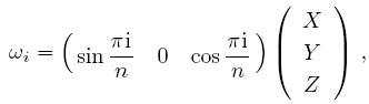
where $\omega_{i}$, $i=1,3,\ldots, N-1$ are Alice's measurement operators when Alice's measurement bases selection are $x_i$, and Alice's measurement operators can be represented by $A_{x_i}^{a_i}$. Similarly, $i=2,4, \ldots, N$ are Bob's measurement operators when Bob's measurement bases selection are $y_i$, and Bob's measurement operators can be represented by $B_{y_i}^{b_i}$. Here $X=\sigma_{x}=$ , $Y=\sigma_{y}=$
 , and $Z=\sigma_{z}=$
 are Pauli operators. Specifically, if there are only four measurement bases (i.e. $N=2n=4$), Chain inequality is equal to the CHSH inequality.
, $Y=\sigma_{y}=$, and $Z=\sigma_{z}=$ are Pauli operators. Specifically, if there are only four measurement bases (i.e. $N=2n=4$), Chain inequality is equal to the CHSH inequality.3 Weak Measurement
Quantum weak measurement was proposed by Aharonov, Albert, and Vaidamn in 1988,[19] which was proven to be useful for signal amplification, state tomography, and solving quantum paradoxes.[20-24] Comparing with the projective measurement, quantum weak measurement only introduces small disturbance to quantum system and will not make quantum states collapse entirely. The detailed weak measurement model is demonstrated in Fig. 1.
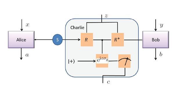
Fig. 1 (Color online) Operating procedure of weak measurement. |
In the weak measurement model, $S$ generates the maximal entanglement state $\Psi_{AB}={(|01\rangle-|10\rangle)}/{\sqrt{2}}$ and sends the two particles to Alice and Bob respectively. After receiving the quantum state, Alice (Bob) selects measurement basis with the random number $x$ ($y$). The weak measurement model Charlie receives the quantum state and applies the operation $R_{z}|0\rangle=|\omega_{z}\rangle$, $R_{z}|1\rangle=|\omega_{z}^{\bot}\rangle$, where $|\omega_{z}\rangle$ and $|\omega_{z}^{\bot}\rangle$ are a new basis in the two-dimensional Hilbert space.
After receiving the quantum state $|1\rangle$, Charlie applies the following control operation $e^{i\varepsilon\sigma_{z}}$ , where $\varepsilon$ is the weak measurement parameter. This process is equal to the operation that carries out collective measurement on the particle sent to Bob and Charlie's state $|+\rangle$, then Alice, Bob, and Charlie measure their quantum states to get the measurement outcomes. By considering Alice, Bob and Charlie as an integer system, the previous $R$ operation can be represented as
, where $\varepsilon$ is the weak measurement parameter. This process is equal to the operation that carries out collective measurement on the particle sent to Bob and Charlie's state $|+\rangle$, then Alice, Bob, and Charlie measure their quantum states to get the measurement outcomes. By considering Alice, Bob and Charlie as an integer system, the previous $R$ operation can be represented as $ U_{1}=I\otimes R_{z}\otimes I\,. $
After the $R$ operation, the weak measurement operation $e^{i\varepsilon\sigma_{z}}$ can be represented as
$ U_{2}=I\otimes |0\rangle \langle0| \otimes I +I\otimes |1\rangle \langle1| \otimes e^{i\varepsilon\sigma_{z}}\,. $
Finally, the last operation can be represented as
$ U_{3}=I\otimes R_{z}^{+}\otimes I\,. $
Combining these three steps, we can get
$ \qquad U=U_{3}U_{2}U_{1} =I\otimes \pi_{B}^{+Z}\otimes I +I\otimes \pi_{B}^{-Z}\otimes e^{i \varepsilon \sigma_{z}}\,, $
where $\pi_{B}^{+Z}=|\omega_{z}\rangle\langle\omega_{z}|$ and $ \pi_{B}^{-Z}=|\omega_{z}^{\bot}\rangle\langle\omega_{z}^{\bot}|$.
The density matrix of the initial state about Alice, Bob and Charlie's quantum system can be given by $\rho_{ABC}=\rho_{AB}\otimes |+\rangle\langle+|_{C}$, where Alice and Bob's systems have no correlation with Charlie's system. The density matrix of Alice and Bob's system is $\rho_{AB}=({1}/{2})P(|0\rangle|1\rangle-|1\rangle|0\rangle)=({1}/{2})P(|\omega_{z}\rangle |\omega_{z}^{\bot}\rangle-|\omega_{z}^{\bot}\rangle|\omega_{z}\rangle)$ where $P|x\rangle=|x\rangle\langle x|$. After the corresponding quantum state evolution, the density matrix of Alice, Bob and Charlie's quantum system can be given by
$ \rho_{ABC}^{'}=U\rho_{ABC}U^{\dagger} =(I\otimes \pi_{B}^{+Z}\otimes I+I\otimes \pi_{B}^{-Z}\otimes e^{i \varepsilon \sigma_{z}})\rho_{ABC}(I\otimes \pi_{B}^{+Z} \otimes I+I\otimes \pi_{B}^{-Z}\otimes e^{i \varepsilon \sigma_{z}})^{\dagger}\,. $
4 Chain Inequality with Weak Measurement
After receiving the quantum state $\rho_{AB}$, Alice and Bob firstly calculate their own Bell inequality according to their measurement outcomes. Similarly, Alice and Charlie also can calculate their Bell inequality by receiving the quantum state $\rho_{AC}$. If the two Bell inequality values both violate classical upper bound, we can realize the double Bell inequality violation.
The number of measurement bases $N$ is determined by Alice and Bob, which have different Bell inequality values. Note that, the measurement bases selected by Charlie are equal to Bob's measurement bases selection, which can be represented by $C^{c}$, $c$ is Charlie's measurement outcome.
When applying the weak measurement model with the Chain inequality, we calculate the Chain inequality about Alice and Bob's systems to get the inequality value $I_{AB}$. Similarly, we can calculate the Chain inequality about Alice and Charlie's systems to get the inequality value $I_{AC}$. To calculate the Chain inequality value, we apply the following equation
$$ I _{AB}=C(x_{1},y_{2})+C(y_{2},x_{3})+C(x_{3},y_{4})+\cdots +C(x_{N-1},y_{N}) -C(y_{N},x_{1}) (C(x_i,y_j)=\sum\limits_{a_i,b_j} a_ib_jP(a_i,b_j|x_i,y_j)) $$
represents the Chain inequality value about Alice and Bob's quantum systems with input random number $x_i$ and $y_j$ and measurement outcomes $a_i$ and $b_j$.
$$ I _{AC}=C(x_{1},z_{2})+C(z_{2},x_{3})+C(x_{3},z_{4}) +\cdots+C(x_{N-1},z_{N}) -C(z_{N},x_{1}) (C(x_i,z_k)=\sum\limits_{a_i,c_k} a_ic_kP(a_i,c_k|x_i,z_k)) $$
represents the Chain inequality value about Alice and Charlie's quantum systems with input random number $x_i$ and $z_k$ and measurement outcomes $a_i$ and $c_k$.
To calculate the Chain inequality value, the conditional probabilities between Alice and Bob can be given by
$ \qquad P(a_ib_j|x_iy_j)=\sum\limits_{z_k}P(z_k) {\rm tr}(A_{x_i}^{a_i}B_{y_j}^{b_j}\rho_{AB}^{'}(z_k))\,. $
Correspondingly, the conditional probabilities between Alice and Charlie can be given by
$ P(a_ic_k|x_iz_k)={\rm tr}(A_{x_i}^{a_i}C^{c_k}\rho_{AC}^{'}(z_k))\,. $
The corresponding density matrices are $\rho_{AB}^{'}(z_k)={\rm tr}_{C}(\rho_{ABC}^{'})$ and $\rho_{AC}^{'}(z_k)={\rm tr}_{B}(\rho_{ABC}^{'})$. The main difficulty to estimate the Chain inequality is to calculate the conditional probabilities $P(a_ib_j|x_iy_j)$ and $P(a_ic_k|x_iz_k)$. The precise density matrix can be respectively given by
$ \rho_{ABC}^{'}=\pi_{B}^{+Z}\rho_{ABC}\pi_{B}^{+Z}+ \pi_{B}^{+Z}\rho_{ABC}\pi_{B}^{-Z}(e^{-i\varepsilon\sigma_{z}})_{C} +\pi_{B}^{-Z}(e^{i\varepsilon\sigma_{z}})\rho_{ABC}\pi_{B}^{+Z} +\pi_{B}^{-Z}(e^{i\varepsilon\sigma_{z}})\rho_{ABC}\pi_{B}^{-Z} \times(e^{-i\varepsilon\sigma_{z}})\,, $
then
$ \rho_{AB}^{'}(z_k)={\rm tr}_{C}(\rho_{ABC}^{'}) =\pi_{B}^{+Z}\rho_{AB}\pi_{B}^{+Z}+\pi_{B}^{+Z}\rho_{AB} \pi_{B}^{-Z}\cos \varepsilon +\pi_{B}^{-Z}\rho_{AB}\pi_{B}^{+Z}\cos \varepsilon +\pi_{B}^{-Z}\rho_{AB}\pi_{B}^{-Z} =\rho_{AB}\cos\varepsilon+(1-\cos\varepsilon)(\pi_{B}^{+Z} \rho_{AB}\pi_{B}^{+Z} +\pi_{B}^{-Z}\rho_{AB}\pi_{B}^{-Z})\,. $
Substituting Eq. (11) into Eq. (8),
$ P(a_ib_j|x_iy_j) =\sum\limits_{z_k}P(z_k){\rm tr}(A_{x_i}^{a_i}B_{y_j}^{b_j}\rho_{AB}^{'}(z_k)) =\sum\limits_{z_k}P(z_k){\rm tr}(|\mu_{x_i}^{a_i} \rangle\langle\mu_{x_i}^{a_i}||\theta_{y_j}^{b_j}\rangle\langle \theta_{y_j}^{b_j}|(\rho_{AB}\cos\varepsilon +(1-\cos\varepsilon)(\pi_{B}^{+Z}\rho_{AB}\pi_{B}^{+Z} +\pi_{B}^{-Z}\rho_{AB}\pi_{B}^{-Z}))) =\frac{1}{4}\sum\limits_{z_k}P(z_k)(\cos\varepsilon(1-a_ib_j (\mu_{x_i}\cdot\theta_{y_j})) +(1-\cos\varepsilon) (1-a_ib_j(\mu_{x_i}\cdot\eta_{z_k})(\theta_{y_j}\cdot\eta_{z_k})))\,. $
We assume that Alice, Bob and Charlie apply the optimal measurement to reach the upper bound value of the Chain inequality, the corresponding Pauli operators can be given by $\mu_{x_i}$, $\theta_{y_j}$, and $\eta_{z_k}$.
Then we have the Chain inequality value between Alice and Bob is
$ I_{AB}=\cos\frac{\pi}{N}((N-2)\cos\varepsilon+2)\,. $
Similarly, the Chain inequality value between Alice and Charlie is given by
$ I_{AC}=N\cos\frac{\pi}{N}\sin^{2}\varepsilon\,. $
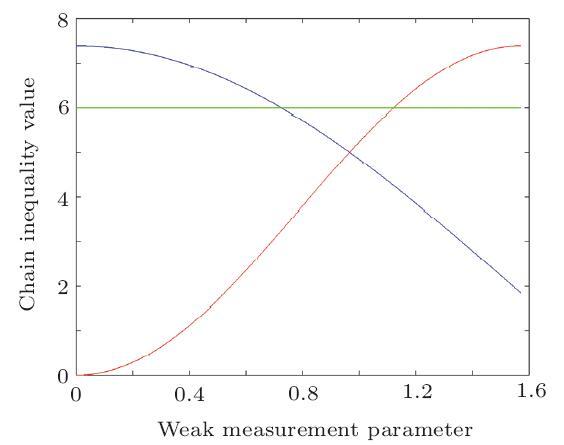
Note that $\varepsilon=0$ indicates $I_{AB}=N\cos({\pi}/{N})$ and $I_{AC}=0$, which demonstrates that Charlie's quantum state has no interaction with Bob's system. In this case, only $I_{AB}$ violates the classical upper bound $N-2$. In the case of $\varepsilon={\pi}/{2}$, we can get $I_{AB}=2\cos{\pi}/{N}$ and $I_{AC}=N\cos{\pi}/{N}$, which demonstrates that only Charlie and Bob's system can violate the classical upper bound.
Figures 2, 3, and 4 illustrate the Chain inequality values $I_{AB}$ and $I_{AC}$ with different weak measurement parameters $\varepsilon$, where the blue line represents the Chain inequality value $I_{AB}$, the red line represents the Chain inequality value $I_{AC}$, the green curve represents the classical upper bound of different Chain inequalities.
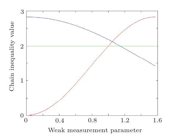
Fig. 2 (Color online) Two measurement basis with $n$=2. The blue line represents the Chain inequality value $I_{AB}$, the red line represents the Chain inequality value $I_{AC}$, the green curve represents the classical upper bound of Chain inequalities. |
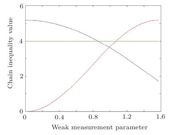
Fig. 3 (Color online) Two measurement basis with $n$=3. The blue line represents the Chain inequality value $I_{AB}$, the red line represents the Chain inequality value $I_{AC}$, the green curve represents the classical upper bound of Chain inequalities. |
Fig. 4 (Color online) Two measurement basis with $n$=4. The blue line represents the Chain inequality value $I_{AB}$, the red line represents the Chain inequality value $I_{AC}$, the green curve represents the classical upper bound of Chain inequalities. |
We can figure out that the inequality values $I_{AB}$ and $I_{AC}$ can both violate the classical upper bound value in the case of $n=2$ with the appropriate weak measurement parameter. In the case of $n\geq3$, the Chain inequality can not realize the double classical upper bound violation. However, we can realize the inequality value $I_{AB}$ or $I_{AC}$ violate the classical upper bound with different weak measurement parameters. Thus our analysis model may be applied to analyze the device independent protocols with the network environment.
5 Conclusion
In conclusion, we propose the weak measurement model to analyze the Chain inequality, and the double inequality violation can be observed in the case of $n=2$. In the case of $n\geq3$, two different parties can respectively realize the Chain inequality violation with different weak measurement parameters. The analysis results demonstrate that weak measurement may have significant applications in multi observer quantum information theory. More precisely, our analysis model may be applied to analyze the device independent quantum information protocols in the network environment, which can be utilized to generate high efficiency device independent random numbers. On the other side, our analysis result also provides tremendous motivation for further experimental research.