


1 Introduction
Since Anderson's pioneering work on the interplay of quantum mechanics and disorder, localized system has been extensively studied over the past several decades.[1] Arising naturally in real systems, disorder could influence the transport property of electrons in solids, which show fascinating behaviors.[2-6] It was demonstrated that, in one-dimensional system, arbitrary small disorder strength will cause exponential localization of all the eigenstates in the band, which was confirmed by numerical simulation methods.[7-8] Among these studies, most efforts are focused on the discrete Hamiltonian,
$ H=\sum_{i}\epsilon_i c_{i}^{†}c_i+\sum_{j\neq i}t_{ji}c_j^{†}c_i\,, $
where $\epsilon_i$ is the on-site energy and $t_{ji}$ is the hopping energy from the $i$-th site to the $j$-th site. Varying from system to system, we can basically divide them into diagonal or off-diagonal and correlated or non-correlated disorder systems.[9-10] In this paper, we aim at one-dimensional system with diagonal and uncorrelated disorder in which only hoppings between the nearest sites are considered.
For previous models, it was found that the Lyapunov exponent behaves anomalously near
the band center,[11] which is deviated from Thouless formula.[12] The perturbation method has been applied to deal with this mysterious region in the weak or strong disorder limits.[13-15] Derrida and Gardner developed a disorder expansion method for weak disorder in Ref. [14], which recovered the anomaly near band center and band edge and predicted that similar anomaly exists in the vicinity of $E=2\cos\alpha\pi$, with $\alpha$ to be a rational number. Then it was confirmed in Ref. [16], where they obtained the Lyapunov exponent in two limiting cases around band center,
$ \gamma=\frac{\sigma^2\pi}{8 K^2(1/\sqrt{2})} \Big[1+O\Big(\frac{E}{\sigma^2}\Big)\Big]\, , \quad \frac{E}{\sigma^2}\ll 1 \,, \\ \gamma=\frac{\sigma^2}{8}\Big[1- \frac{3}{16} \Big(\frac{\sigma^2}{E}\Big)^2 + \cdots \Big]\,, \quad \frac{\sigma^2}{E}\ll 1 \,, $
where $K(1/\sqrt2)$ is the complete elliptic function of the first kind, $E$ and $\sigma^2$ are the energy and disorder strength. Due to its sensitivity to energy and disorder strength, general analytical treatment to the whole neighborhood of band center has not been found yet. An analytical expression will be provided to relate the above two limiting cases in this work.
As discussed above, analytical formula performs well in the anomalous and traditional area respectively. Although it seems hard to connect them by a unified description, numerical calculation indicates that it could be possible to give formula except the band edge anomalous region.[17] In this work, by making use of the parametrization method proposed in a previous work,[18] we develop a new approach to obtain the invariant distribution coincided with the result given by Hamiltonian map method in Ref. [19]. This paper is organized as follows. In Sec. 2, we briefly review the parametrization method. In Sec. 3, by expanding the integral equation in terms of $E$ and $\sigma^2$, we derive a corresponding differential equation and invariant distribution. Then, the solution of this equation is used to obtain information in two limiting cases. In Sec. 4, a Padé approximation formula is given to describe the behavior of Lyapunov exponent for the whole neighborhood of band center.
2 Parametrization Method
We start by introducing the parametrization method in this section for the Schrödinger equation of one-dimensional diagonal disorder Anderson system,
$ \psi_{i-1}+\psi_{i+1}=(E-\epsilon_i)\psi_i \,. $
The energy $E$ of an electron and the on-site energy ${\epsilon_i}$ of disorder system have been rescaled by the nearest neighbor hopping energy. $\{\epsilon_i\}$ are independent to each other and obey an identical distribution $p_\epsilon (\epsilon)$. In this study we assume that the random potential $\epsilon_i$ with a zero mean $<\epsilon>=0$, a nonzero variance $<\epsilon^2>=\sigma^2$, and an even distribution $p_\epsilon (-\epsilon) = p_\epsilon (\epsilon)$. For this purpose we use a standard distribution for on-site energy in our calculation,
$ p_\epsilon (\epsilon)=\frac{1}{\sigma\sqrt{\pi}} \exp\Big(-\frac{\epsilon^2}{\sigma^2}\Big) \,. $
The Schrödinger equation can be rewritten in transfer matrix $ T_i$ as
$ \Psi_{i+1}= \begin{pmatrix} \psi_{i+1}\\ \psi_{i} \end{pmatrix} =\begin{pmatrix}E-\epsilon_i & -1\\ 1 & 0\end{pmatrix} \begin{pmatrix} \psi_i \\ \psi_{i-1}\end{pmatrix}={ T}_i\Psi_{i} \,. $
As the authors performed in Ref. [18], we define the total transfer matrix $ M_L={ T_L}{ T_{L-1}}\ldots{ T_1}$, and parametrize it by two real parameters $\theta_L$ and $\lambda_L$.
$ U(\theta_L) M_L M_L^t U(-\theta_L)=\begin{pmatrix} e^{\lambda_L}& \\ & e^{-\lambda_L}\end{pmatrix} , $
where $ M_L^t$ is the transpose matrix of $ M_L$, and $ U(\theta_L)$ is
$ U(\theta_L)=\begin{pmatrix}\cos\theta_L &-\sin\theta_L\\\sin\theta_L&\cos\theta_L\end{pmatrix} . $
Utilizing the definition of $ M_{L}$ and $ M_{L+1}$, we obtain the recursion relation of $\theta_L$,
$ \tan\theta_{L+1}=\frac{1}{E-\epsilon_{L+1}-\tan\theta_L}\,. $
This recursion relation gives the exact integral equation for the stationary distribution function $\rho(\theta)$ of the random number $\theta_L$,
$ \rho(\theta)\sin^2\theta=\int_{-\infty}^{\infty} p_\epsilon (\epsilon)\rho(\theta_1)\cos^2\theta_1 d\epsilon\,, $
here $\theta_1$ is a function of $\theta$, $\tan\theta_1=E-\epsilon-{1}/{\tan\theta}$.
The Lyapunov exponent is the average of $(1/2) (\lambda_{L+1}-\lambda_{L})$, where $\lambda_{L}$ is defined in Eq. (6). $\gamma$ can be expressed by a normalized $\rho(\theta)$ in
$ \gamma = \frac{1}{2}\int_{-\pi/2}^{\pi/2} d\theta \int_{-\infty}^{\infty} d\epsilon \rho(\theta)p_{\epsilon}(\epsilon) \\ \hphantom{\gamma=} \times \ln [1+(E-\epsilon)^2\cos^2\theta -(E-\epsilon)\sin2\theta]\, . $
It is equivalent to the formula $\gamma=\int \rho(\theta)\ln|\tan\theta|$ used in Refs. [13--14]. This integral equation and Lyapunov exponent are valid for all energies and disorder strengths.[18] We will use Eq. (10) in weak disorder and band center case at the last part of next section, as it can be expanded in terms of $\sigma^2$ and $E$ because of the direct relation to both distribution $p_{\epsilon}(\epsilon)$ and energy $E$.
When the variance $\sigma^2\rightarrow 0$, the distribution of $\theta$ is determined only by the distribution of $\theta_1$. The distribution of random potential becomes a delta function and it yields
$ \rho(\theta)\sin^2\theta = \rho(\theta_1)\cos^2\theta_1\,, \quad \tan\theta_1 = E-\frac{1}{\tan\theta} \,. $
Equation (11) gives the equation that the distribution function has to satisfy in the limiting case $\sigma^2 \to 0$. The solution of this equation is $\rho(\theta)=1/(1-({E}/{2})\sin 2\theta)$ for in-band energies.
In the limit $\sigma^2 \to 0$, if we consider next the band center limit $E\rightarrow 0$, Eq. (11) reduces to
$ \rho(\theta)\sin^2\theta=\rho\Big(\theta-\frac{\pi}{2}\Big)\sin^2\theta \,. $
It shows that if any distribution function satisfies $\rho(\theta)=\rho(\theta-{\pi}/{2})$, it may be a stationary distribution. There are many distributions under this symmetry. Then $\gamma$ is not uniquely defined, and this is not true for a disordered system. Such a degenerate phenomenon of $\rho(\theta)$ distribution has been discussed in Ref. [13]. It is the mathematical reason for the zero energy anomaly. At any $E=2\cos\alpha\pi$ with $\alpha$ to be a rational number, however, anomaly in $\gamma$ could rise in orders higher than $\sigma^2$, as a recent study[19] demonstrated. We will go to the next order of $\sigma^2$ for the exact integration equation Eq. (9) to resolve the unique $\rho(\theta)$ distribution under $E\to 0$ in next section.
3 $E/\sigma^2$ Dependence of Zero Energy Anomaly
In this section we write out the differential equation of distribution from the exact integration equation Eq. (9) in weak disorder for band center anomaly, formulate its solution, and expand the Lyapunov exponent $\gamma$ to the leading corrections for $\sigma^2/E \to 0$ and $\sigma^2/E \to \infty$.
We approach the solution for band center by iterating this recursive integration equation twice
$ \rho({\theta}) = \int_{-\infty}^{\infty}\int_{-\infty}^{\infty} d\epsilon_1 d\epsilon_2 \frac{ \exp[ - ({\epsilon_1^2+\epsilon_2^2})/{\sigma^2}]} {\pi \sigma^2} \\ \times\frac{ \sin^2\theta_2 \rho({\theta_2}) } {\tan^2\theta_1 \tan^2\theta_2 \sin^2\theta}\,, $
where $\tan\theta_1=E-\epsilon_1-{1}/{\tan\theta}$, and $\tan\theta_2=E-\epsilon_2-{1}/{\tan\theta_1}$. Then it is possible to calculate the stationary distribution in the limits $E\rightarrow 0$, $\sigma^2\rightarrow 0$. Since $\theta_2$ will be sufficiently close to $\theta$, $\rho(\theta_2)$ can be expanded around $\theta$, and the integration equation can be written into a differential equation of $\rho(\theta)$.
We expand Eq. (13) in powers of $E$ and $\sigma^2$
$ \rho(\theta) = \rho(\theta)+E \rho'(\theta) +\sigma^2\Big[\frac{\sin^4\theta+ \cos^4\theta}{2} \rho^{\prime\prime}(\theta) -\frac34\sin4\theta \rho'(\theta) -\cos4\theta \rho(\theta)\Big] + O(E\sigma^2)+O(E^2)+O(\sigma^4) \,. $
Let us neglect higher order terms of $\sigma^2$ and $E$. Then by defining $x={E}/{\sigma^2}$, we get
$ \frac{3+\cos4\theta}{8}\rho^{\prime\prime}(\theta) -\Big(\frac{3 \sin4\theta }{4} -x\Big)\rho'(\theta) -\cos4\theta\, \rho(\theta)=0\,. $
The normalized distribution obtained as the solution of Eq. (15) in this study is
$ \rho(\theta)= \frac{1}{N(x)} \frac{2\sqrt2 x}{1-e^{-\sqrt2 \pi x}} \frac{1}{\sqrt{3+\cos4\theta}} \int_{0}^{\pi/2} d\theta_1 \\ \times\frac{ \exp\big[-\frac{x}{\sqrt2}\big(4\theta_1 -2\tan^{-1}\frac{\sin4(\theta_1-\theta)} {\cos4(\theta_1-\theta) +2\sqrt2+3} -2\tan^{-1}\frac{\sin4\theta}{\cos4\theta+2\sqrt2+3}\big)\big]} {\sqrt{3+\cos4(\theta_1-\theta)}}\,, $
where $N(x)$ is the normalization factor. We include a factor ${ 2\sqrt2 x}/{1-e^{-\sqrt2 \pi x}}$ to scale $N(x)$ to the order of $1$. This solution is continuous, periodic $\rho(\theta+\pi/2)=\rho(\theta)$, and have obvious $x$-dependent properties $\rho(\theta,-x)=\rho(-\theta,x)$ and $N(-x)=N(x)$. We denote the exponential part in the distribution by a function
$$ C(\theta,\theta_1)= 4\theta_1 -2\tan^{-1}\frac{\sin4(\theta_1-\theta)} {\cos4(\theta_1-\theta)+2\sqrt2+3} \\ -2\tan^{-1}\frac{\sin4\theta}{\cos4\theta+2\sqrt2+3}\,, $$
which will be used in perturbation expansion later.
$$ F(\theta)=\int_0^{\theta}\frac{1}{3+\cos4\phi}d\phi $$
is constructed by piecewise function since a constant $n\pi$ must be included according to the magnitude of $\theta$ to keep the periodicity and continuity of $\rho(\theta)$. This integer $n$ was removed by a monotonic function in our solution
$$ F(\theta) = \frac{1}{4 \sqrt{2}}\Big( 2\theta -\tan^{-1}\frac{\sin4\theta}{\cos4\theta+2\sqrt2+3} \Big)\, . $$
Moreover, the normalized distribution and normalizing factor given in Eq. (26) and Eq. (27) in Ref. [21] missed a factor ${1}/({1-e^{-\sqrt 2 \pi x}})$ before the second integration. Therefore a plot of $\rho(\theta)$ based on these equations will be non-continuous.
When the energy and disorder strength are sufficiently small, the leading order of Lyapunov exponent given in Eq. (10) can be obtained,
$ \gamma \!=\!\frac{\sigma^2}{2}\int_{-\pi/2}^{\pi/2} \! d \theta \rho(\theta)\Big(\frac{1+2\cos2\theta+\cos4\theta}{4}-x\sin2\theta\Big) . $
Implementing a quasi-degenerate perturbation method, Goldhirsch and Noskowicz[13] obtained the result for the limiting cases of $|x|\ll1$ and $|x|\gg1$ respectively. We give the first correction terms through the exact distribution in Eq. (16) in the following.
In the limit of $|x|\ll 1$, the normalization factor $N(x)$ is
$ N(x) = \frac{K^2(1/\sqrt{2})}{\pi} + N_{02} x^2 + \cdots \,, \\ N_{02}= \int_{-\pi/2}^{\pi/2}d \theta \int_{0}^{\pi/2}d \theta_1 \\ \hphantom{ N_{02}=}\times \frac{ ({\pi }/{3}) + C(\theta,\theta_1) + { ( C(\theta,\theta_1) )^2 }/{2\pi}} { \sqrt{ (\cos 4 \theta +3) (\cos (4 (\theta_1-\theta))+3)} } \,, $
where the long expression for $C(\theta,\theta_1)$ was introduced after Eq. (16). We can numerically integrate out the coefficient and $N(x)=1.09422 + 0.00814695 x^2+\cdots$ And the leading correction of Lyapunov exponent is
$$ \gamma= \frac{\sigma^2}{N(x)}\Big(18+ G_{02} x^2+\cdots\Big)\,, $$
$ G_{02}= \int_{-\pi/2}^{\pi/2}d \theta \int_{0}^{\pi/2}d \theta_1 \frac{1} {\sqrt{\cos 4 \theta +3} \sqrt{\cos (4 (\theta_1-\theta))+3}} \\ \hphantom{{G_{02}}}\times \Big[ \frac{1+2\cos2\theta+\cos4\theta}{4} \Big( \frac{\pi }{6} - \frac{ C(\theta,\theta_1) }{2}+ \frac{ ( C(\theta,\theta_1) )^2 }{\pi} \Big) - \frac{ (\pi - C(\theta,\theta_1)) \sin 2 \theta }{\sqrt{2} \pi } \Big]\, . $
We can numerically integrate out the coefficient $G_{02}$ and $\gamma= ({\sigma^2}/{N(x)})(1/8+ 0.00675927 x^2+\cdots)$.
Using the above coefficients, Eq. (19) can be rewritten as
$ \gamma(x) =\gamma(0)[1+0.0466287 x^2+O(x^4)]\,. $
The zeroth order term in $x$, $\gamma(0)= {\pi \sigma^2}/{8 K^2(1/\sqrt{2})}=0.114237\sigma^2$, is in agreement with the known result in Ref. [13--14]. To our knowledge, there is no result of the leading correction term in previous studies.
Then we also explicitly show the leading terms in the limit of $|x|\gg 1$. They are analytically obtained through the distribution Eq. (16)
$ N(x) = \frac{\pi }{2 \sqrt{2}} -\frac{\pi}{64 \sqrt{2}} \frac{1}{x^2} + \cdots\,, \\ \gamma(x)= \frac{\sigma^2}{N(x)} \Big( \frac{\pi }{16 \sqrt{2}}-\frac{7 \pi}{512 \sqrt{2}} \frac{1}{x^2} +\cdots \Big)\,, $
and so
$ \gamma(x) = \gamma(\infty) \Big(1-\frac{3}{16} \frac{1}{x^2}+\cdots\Big)\, , $
with $\gamma(\infty) = \sigma^2/8$. Unlike in the small $x$ limit, the first correction term in the large $x$ limit has been obtained in Refs. [13--14]. In Ref. [21] this leading correction term was elegantly derived directly from the differential equation Eq. (15).
Although we only have limited analytical method for the properties of $\gamma(x)$, we can investigate the band center anomaly in the full $x$ range by numerical integration. We will demonstrate the full range behavior of stationary distribution and localization in next section.
4 Discussion on Band Center Anomaly
The energy is small for band center anomaly, so that the expansion can be used to obtain a solution for the stationary distribution. It is not well understood of $\rho(\theta)$ given by Eq. (16) for band center anomaly in weakly disordered chain. In Fig. 1, we plot numerical value of the normalization factor $N(x)$ for the invariant distribution. It shows $N(x)$ is of order $1$. We included a scaling factor in $\rho(\theta)$ and scaled $N(x)$ to order $1$ from $x \to 0$ to $x \to \infty$, but it is hard to see in Fig. 1 what kind of function of $x$ it is. Without a simple analytical expression for $N(x)$, one cannot give a full $x$ range description for $\gamma(x)$. At the end of this section, we will give a Padé approximation for $\gamma(x)$ for any magnitude of $x$.
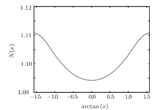
Fig. 1 The normalization factor $ N(x)$. The full line is the normalization factor in Eq. (16), $x=E/\sigma^2$, and the horizontal axis in $\arctan(x)$ is used to show all possible magnitude of $x$. |
Let us return to the differential equation. The ratio $x$ is free to choose and that is the primary dilemma we encounter. Considering $x\ll 1$, if we neglect the terms with respect to $x$, the differential equation Eq. (15) becomes
$ \frac{3+\cos4\theta}{8}\rho^{\prime\prime}(\theta)-\frac34\sin4\theta \rho'(\theta) -\cos4\theta \rho(\theta)=0 \,, $
with the normalized solution for distribution[13]
$ \rho(\theta)=\frac{1}{K(1/\sqrt2)\sqrt{3+\cos4\theta}} \,. $
When $x$ approaches infinity, Eq. (15) reduces to
$ \rho'(\theta)=0\,, $
which means $\rho(\theta)$ is a constant, $\rho(\theta)={1}/{\pi}$.
In Fig. 2, we plot the invariant distribution function $\rho(\theta)$ according to Eq. (16). It demonstrates that, as $x\rightarrow 0$, the distributions collapse on Eq. (24). As $x$ getting close to infinity, the distribution function gradually becomes flat and the amplitude of oscillation is decreasing. These properties of the solution for general $x$ are in agreement with above analysis for the limiting cases discussed.
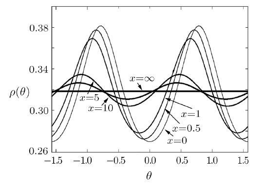
Fig. 2 Invariant distribution $\rho(\theta)$ for $x=0$, $0.5$, $1$,$5$, $10$, and $\infty$, respectively. The lines with oscillation amplitudes from big to small are in correspondence with the magnitude of $x$ from small to big, one by one. The flat $\rho(\theta)$ line is of $E/\sigma^2=\infty$. |
In Fig. 3 we plot the numerical values of Lyapunov exponent $\gamma(x)$ in Eq. (17) for all possible $x$. We plot in the same figure also the asymptotic behaviors of Lyapunov exponent for $x\to 0$ and $x\to\infty$ according to Eqs. (20) and (22). As shown in Fig. 3, the leading correction terms in the asymptotic series can give a good description for a certain range when $x$ is big or small. An expression for $\gamma(x)$ for the middle magnitude $x$ should be interesting.
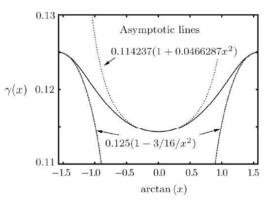
Fig. 3 Lyapunov exponent $\gamma(x)$ in unit of $\sigma^2$. The full line is the Lyapunov exponent in Eq. (17). The dashed and dotted lines are the asymptotic behavior upto the first correction term for $x\to\infty$ and $x\to 0$, respectively. |
In Ref. [17], such an expression has been obtained by fitting numerically obtained $\gamma(x)$ in that work,
$$ \gamma(x)=\gamma_p\Big[1-\frac{0.086}{1+(x/1.426)^2}+\cdots\Big]\,, $$
where $\gamma_p = {\sigma^2}/{8(1-E^2/4)}$ is the perturbation result first obtained by Thouless.[12] In Fig. 3 we will not be able to resolve the difference between the full line and this fitting curve if we plot them together. This fitting matches the small $x$ region well and the coefficient of $x^2$ correction term has two accurate digits. However, the asymptotic behavior in $x\to \infty$ is wrong.
At the end of this section, we give a Padé approximation for $\gamma(x)$ for any magnitude of $x$ for practical use. For describing the whole anomalous region in the vicinity of band center, one can write down a rational Padé approximation without free parameters,
$ \gamma_{\rm pade}= \frac{\gamma(0)+0.310615\sigma^2 x^2+\gamma(\infty)x^4} {1+2.67242 x^2+x^4}\, . $
Since $\gamma(0)$ and $\gamma(\infty)$ have been already found, the $-3/16$ and 0.046 628 7 coefficients in leading correction terms in Eq. (20) and Eq. (22) completely fixed the coefficients of $x^2$ terms in this Padé approximation.
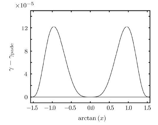
In Fig. 4, the difference between $\gamma(x)$ and the Padé approximation formula is plotted. It shows that the approximation is very good when $x$ is big or small. The maximum difference is of order $1\times 10^{-4}$, which appears at a middle magnitude $x$. $\gamma(x)/\sigma^2$ has been shown to be of order $0.1$ in Fig. 3. Now we have an approximated expression with at least four accurate digits for $\gamma(x)$.
Fig. 4 The difference between the numerical values of Lyapunov exponent $\gamma(x)$ in Eq. (17) and its Padé approximation $\gamma_{\rm pade}(x)$ in Eq. (26). The full line is the difference in unit of $\sigma^2$. |
In conclusion, we analytically studied the properties of the Lyapunov expoent in the vicinity of $E=0$ for one-dimensional Anderson model with diagonal random potential. By implementing the parametrization method, we obtained the recursion integration equation for invariant distribution function. In the weak disorder and band center case, a differential equation involving the ratio of energy and disorder strength $x=E/\sigma^2$ is derived. The solution of this equation is given to show that this ratio $x$ directly affects the invariant distribution as well as the behavior of Lyapunov exponent. Finally, we presented a Padé approximation formula which could not only reproduce the Thouless formula and anomaly within their valid range respectively, but also provide a transparent way to describe the transition. As it was pointed out in Ref. [17], higher order terms in $x$ exist, a simple analytical function of $x$ is still to be found for Lyapunov exponent.
Acknowledgments
The authors thank Profs. Zhou Sen, Xu Yuan-Yuan, Wu Long-Biao, Zhou Hao, Huang Yun-Peng for discussions.