


1 Introduction
The Chen-Lee-Liu equation
$ {\rm i}q_{t}+q_{xx}+{\rm i}|q|^{2}q_{x}=0\,, $
was introduced as an integrable model at 1979 by inverse scattering method,[1] which is also now called the second-type derivative nonlinear Schrödinger (DNLSII) equation. This equation governs the propagation of the optical pulse involving self-steepening but without self-phase-modulation, which has been validated by an optical experiment at 2007.[2] Thus, like the well-known nonlinear Schrödinger (NLS) equation, the DNLSII is also a real and important physical model, which deserves further deep studies in the future.
Except the DNLSII equation, there exists another type of the derivative NLS equations, i.e., the DNLSI equation
$$ {\rm i}\hat{q}_t+\hat{q}_{xx}+{\rm i}(|\hat{q}|^2\hat{q})_x=0\,. $$
$ q=\hat{q}\exp\left(\dfrac{{\rm i}}{2}\int^x|\hat{q}|^2{\rm d}x\right)\,. $
The transformation in Eq. (2) can generate formally a new solution of the DNLSII from a known solutions of the DNLSI.[5] However, the integral in the left of Eq. (2) is not calculable explicitly in general cases including multi-soliton, and this fact results in a remarkable difficulty to get explicit solutions of the former from the later. This difficulty vastly loses the power of this transformation. So it is necessary to study solutions of two equations separately.
The DNLSII equation has been studied by the bilinear method, and the formula of multi-soliton is given in Refs. [6-7]. Recently, our group constructed the Darboux transformation (DT) of DNLSII equation, and utilized successfully it to get the breather, rogue wave, and multi-rogue wave solutions.[8] In this paper, we shall study the positon solution, breather-positon (b-positon) solution of the DNLSII equation, and the decomposition of positon solution.
The positon solution was firstly introduced for Korteweg-de Vries (KdV) equation by Matveev in 1992,[9] and was quickly extended to other nonlinear integrable equations, such as the modified KdV (mKdV) equation,[10] the sine-Gordon equation,[11] the Toda-lattice,[12] and so on.[13-14] Positon is a long-range analogue of soliton, and the connection between soliton, breather and positon is displayed in Ref. [15]. Further, the positon solution is completely transparent to other interacting nonlinear waves, and two positons remain unchange after mutual collision.[16-17]
The b-positon solution[18] is similar to the positon solution as a result of the degeneration of eigenvalues in them (i.e., $\lambda_i\rightarrow \lambda_1$), except a nonzero boundary condition. Recently, the b-positons are suggested to be excellent approximate representatives of the higher-order rogue wave generated in an optical fiber[18] because of their good stability. Thus, the study of the b-positon of the DNLSII equation is useful to generate higher-order rogue wave in an optical system involving self-steepening without self-phase-modulation.
There are two aims in the article. The first to construct the positons and discuss their decomposition. We shall display a general method to split positon into solitons with a "hase shift", which is a function of time $t$. The second is to construct the b-positon solutions, which will be useful to formulate rogue wave in optical system. The organization of this paper is as follows: In Sec. 2, we give the determinant representation of the positons by the degenerate DT and their decomposition, and an explicit form of variable "hase shift" is given. Further, from the nonzero boundary condition, we generate the b-positon solution. Conclusions are given in the final section.
2 Positons of the Coupled DNLSII Equations
The coupled DNLSII equations are given as
$ {\rm i}q_{t}+q_{xx}+{\rm i}qrq_{x}=0\,,\\ \nonumber {\rm i}r_{t}-r_{xx}+{\rm i}rqr_{x}=0\,. $
This systems admit the following Lax pair[4]
$ \Phi_{x}=P\Phi =\Bigl(-{\rm i}\lambda^{2}+\frac{{\rm i}}{4}qr\Bigr)J\Phi+\lambda M\Phi\,, \\ \Phi_{t}=Q\Phi=\Bigl(-2{\rm i}\lambda^{4}+{\rm i}qr\lambda^{2}+\frac{1}{4}(qr_{x}-rq_{x}) -\frac{{\rm i}}{8}q^{2}r^{2}\Bigr)J\Phi \\ +2\lambda^{3}M\Phi+\lambda W\Phi\,, $
with
If $r=q^*$, then the coupled DNLSII equations give the DNLSII equation (1).
From a zero seed solution $r=q^*=0$, it follows that
$ \Phi_{k}=\left(\begin{matrix} f_{k1}\\ f_{k2} \end{matrix}\right) =\left(\begin{matrix} {\rm e}^{-{\rm i}\lambda_{k}^{2}x-2{\rm i}\lambda_{k}^{4}t}\\ {\rm e}^{{\rm i}\lambda_{k}^{2}x+2{\rm i}\lambda_{k}^{4}t} \end{matrix}\right)\,, $
where $\Phi_k$ is eigenfunction of Lax pair (4) corresponding to $\lambda=\lambda_k$.Let $\lambda_1=\xi_1+{\rm i}\eta_1$ and $\lambda_2=-\lambda_1^*$, based on the DT given in Ref. [8],then the fundamental soliton solution of DNLSII equation is
$ q_{1s}(H)=\frac{-4\xi_{1}\eta_{1}{\rm e}^{-{\rm i}F_{2}}} {\xi_{1}\cosh(F_{1})+{\rm i}\eta_{1}\sinh(F_{1})}\,, $
with
$$ H=4t\xi_{1}^{2}-4t\eta_{1}^{2}+x, \qquad F_{1}=4\xi_{1}\eta_{1}H,\\ F_{2}=4\xi_{1}^{4}t-24\xi_{1}^{2}t\eta_{1}^{2} +2\xi_{1}^{2}x+4\eta_{1}^{4}t-2\eta_{1}^{2}x\,. $$
In the following, we get smooth positon solutions of the DNLSII equation by the degenerate n-fold DT, i.e. set $\lambda_{2k-1}\rightarrow\lambda_1$ in the n-fold DT.[8] Substitute the eigenfunctions $\Phi_{k}$ into the determinant representation of the degenerate n-fold DT, and set $M_{2n}$ and $W_{2n}$ be the forms as appeared in Corollary 1 of Ref. [8] for the case of 2$n$, we can get n-positon of the DNLSII equation in the following form.
Proposition 1 The n-fold DT with a zero seed solution $q=0$ under the degenerate limit $\lambda_{2k-1}\rightarrow\lambda_1(k=1,2,3,\ldots,n)$ generates an n-positon solution of the DNLSII equation, which is given by
$ q_{np}(x,t,\lambda_1)=-2{\rm i}\frac{|M_{2n}|}{|W_{2n}|}\,, $
with two matrices
$ M_{2n}=\left(\frac{\partial^{n_{i}-1}}{\partial\epsilon^{n_{i}-1}}\Bigl|_{\epsilon=0}(U_{2n})_{ik} (\lambda_1+\epsilon)\right)_{2n\times2n} \,,\\ \nonumber W_{2n}=\left(\frac{\partial^{n_{i}-1}}{\partial\epsilon^{n_{i}-1}}\Bigl|_{\epsilon=0}(V_{2n})_{ik} (\lambda_1+\epsilon)\right)_{2n\times2n}\,. $
where $n_{i}=[{(i+1)}/{2}]$, $[i]$ denotes the floor function of $i$. Note that the reduction conditions $\lambda_{2k}=-\lambda_{2k-1}^{*}$ is used in above proposition.
Now we are in position to consider the decomposition of positon solution by applying fundamental soliton. In order to obtain the fundamental positon solution (second order positon), we need consider the second order soliton at first, and then set the eigenvalues going to the same value. Based on degenerated DT given in Eq. (7) and a simple limit $\lambda_3 \rightarrow \lambda_1$, the fundamental (second order) positon solution of DNLSII equation is given by
$ q_{2p}=\dfrac{16{\rm i}\xi_1\eta_1(A_1{\rm e}^{4\xi_1\eta_1 H}+A_2{\rm e}^{12\xi_1\eta_1 H})} {B_0+B_1{\rm e}^{8\xi_1\eta_1 H}+B_0^*{\rm e}^{16\xi_1\eta_1 H}}\exp [-4{\rm i}(\xi_1^4+\eta_1^4-6\xi_1^2\eta_1^2)t +2{\rm i}(\eta_1^2-\xi_1^2)x]\,, $
where
$$ A_1=A_0+\eta_1^3-{\rm i}\xi_1^3,\quad A_2=A_0^*-\eta_1^3-{\rm i}\xi_1^3,\quad A_0=4\xi_1\eta_1^2(\xi_1^2+\eta_1^2)(12\xi_1^2t -4\eta_1^2t+x)-4{\rm i}\xi_1^2\eta_1(\xi_1^2+\eta_1^2)(4\xi_1^2t -12\eta_1^2t+x)\,, \\ B_0=-(\xi_1+{\rm i}\eta_1)({\rm i}\eta_1-\xi_1)^3\,, \\ B_1=1024\xi_1^2\eta_1^2(\xi_1^2+\eta_1^2)^4t^2+512\xi_1^2 \eta_1^2(\xi_1^2-\eta_1^2)(\xi_1^2+\eta_1^2)^2xt+64\xi_1^2 \eta_1^2(\xi_1^2+\eta_1^2)^2x^2 +32{\rm i}\xi_1^2\eta_1^2[(\xi_1^2-\eta_1^2)x+4(\xi_1^4 -6\xi_1^2\eta_1^2+\eta_1^4)t] \\ +2(\xi_1^4+\eta_1^4)\,. $$
As we know, the second order soliton can be viewed as the superposition of two solitons as $t\rightarrow\infty$. Thus, the fundamental positon, a limit case of the second order soliton, should be decomposed asymptotically into two solitons,
$ |q_{2p}|^2\approx |q_{1s}(H+c_1)|^2+|q_{1s}(H-c_1)|^2,\quad t\rightarrow \infty\,. $
Here $c_1$ is the "hase shift" which can be fixed later. Substituting Eqs. (6) and (9) into Eq. (10), and considering the approximation of this equation in the neighbourhood of $H = 0$, it leads to
$ [(\xi_1^2+\eta_1^2){\rm e}^{16\xi_1\eta_1c_1} +2(\xi_1^2-\eta_1^2){\rm e}^{8\xi_1\eta_1c_1} +(\xi_1^2+\eta_1^2)]{\rm e}^{-8\xi_1\eta_1c_1}-2^{12}\xi_1^8 \eta_1^4t^2\approx0\,. $
As we just focus on $c_1$ under the limit $t\rightarrow\infty$, it is a good approximation to solve $c_1$ with leading terms in Eq. (11), namely $ (\xi_1^2+\eta_1^2){\rm e}^{8\xi_1\eta_1c_1} -2^{12}\xi_1^8\eta_1^4t^2\approx0 $, which implies $c_1\approx {1}/{{8\xi_1\eta_1}}\ln {2^{12}\xi_1^8\eta_1^4t^2}/{(\xi_1^2+\eta_1^2)}$. Thus, it is reasonable to select $c_1=\left({1}/{4\xi_1\eta_1}\right)\ln(2^6|t|)$ when $t\rightarrow\infty$.
Proposition As $t\rightarrow\infty$, the fundamental positon solution can be decomposed as
$$ |q_{2p}|^2\approx |q_{1s}(H-c_1)|^2+|q_{1s}(H+c_1)|^2, $$
with a variable "hase shift" $c_1$ defined by
$$ c_1=\dfrac{1}{4\xi_1\eta_1}\ln(2^6|t|). $$
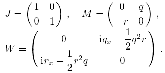
In order to verify the accuracy of our results, we compare the approximate orbits derived by us with the real trajectories of positon, and display it in Fig. 1. In Fig. 1(a), it is easily observed that two trajectories of fundamental positon solution get closer as $t$ goes to $\infty$, so it is reasonable to set that the "hase shift" is dependent of time $t$. In Fig. 1(c), we find that our approximate orbits overlap the real trajectories of fundamental positon very well. Thus, our method about the decomposition of fundamental positon solution is very accurate. Further, our method also works well for higher order positon solution although we do not write out at here.
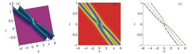
Fig. 1 (Color online) The evolution of the fundamental positon $|q_{2p}|$ of the DNLSII equation with $\xi_{1}=1.3,\eta_{1}=0.7$. (a) The structure of fundamental positon solution. (b) The density profile. (c) The comparsion between the real trajectories of positon and the approximate orbits: The three blue dot lines denote the extreme values of positon solution (including a minimal line); Two dash lines (green and red) denote the approximate orbits. |
Similarly, set $n=3$ in Eq. (7) under limits $\lambda_i\rightarrow \lambda_1~(i=3,5)$, then the three order positon is obtained in a tedious form, and thus is omitted here. We just provide the following decomposition.
Proposition 3 As $t\rightarrow\infty$, the third order positon solution of DNLSII equation can be decomposed as
$$|q_{3p}|^2\approx |q_{1s}(H+c_2)|^2+|q_{1s}(H)|^2+|q_{1s}(H-c_2)|^2\,, $$
with "hase shift" $c_2$ defined by
$$c_2=\dfrac{1}{4\xi_1\eta_1}\ln(2^{11}t^2)\,. $$
Proof The proof is similar to the decomposition for the fundamental positon solution, except that we need to firstly set
$$ |q_{3p}|^2\approx |q_{1s}(H+c_2)|^2 +|q_{1s}(H)|^2+|q_{1s}(H-c_2)|^2\,, \quad t\rightarrow\infty\,, $$
so the detail is omitted.
Remark In Propositions 2 and 3, we call $c_1$ and $c_2$ "hase shift". Because the phase shift of soliton solution is a constant usually, but here $c_i$ $(i=1,2)$ are two functions of $t$. So, the "hase shift" of positon is different from the case of the soliton. Moreover, $q_{1s}(H+\pm c_i)~(i=1,2)$ are not solutions the DNLSII. This is a biggest difference between two kinds of decomposition for solitons and positons.
Similarly, Fig. 2 implies the accuracy of Proposition 3. In Figs. 2(a) and 2(b), the middle dynamic of positon is a straight line, so we set the third order positon includes a soliton without phase shift. Figure 2(c) implies our approximate orbits overlap the real trajectories of third order positon very well.
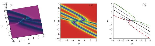
Fig. 2 (Color online) The evolution of the third order positon solution $q_{3p}$ of the DNLSII equation with $\xi_{1}=1.1,\eta_{1}=0.9$. (a) The structure of third order positon solution. (b) The density profile. (c) The comparsion between the real trajectories and approximate orbits for third order positon solution. Four blue dot lines denote the extreme values (including two minimal lines); Two dashes lines (green and red) denote the approximate orbits; The middle black dash-dot line denotes trajectory without phase shift. |
In Ref. [8], the second order breather solution has been considered from the nonzero boundary condition
$ q=c {\rm e}^{i\rho},\quad \rho=ax+bt,\quad b=-a^2-c^2a,\quad a,\,c\in\mathbb{R}\,, $
and the relationship between second order rogue wave and breather solution is discussed. Similar to the fundamental positon solution, in order to obtain the b-positon solution,[18] we have to set that all eigenvalue parameters go to one same value. Here, we just display the dynamic of the second order and the third order b-positon solution, and omit their expressions because of the extra complexity. The second order b-positon is displayed in Fig. 3, and the third order b-positon is displayed in Fig. 4.
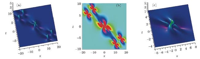
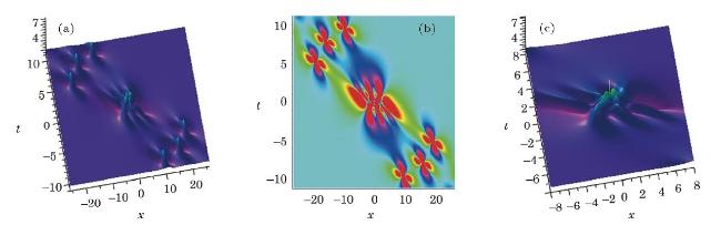
Fig. 3 (Color online) The evolution of fundamental b-position solution of DNLSII equation. (a) The 3-D structure. (b) The density profile. (c) The profile of the central region of (a), which is similar to the second order rogue wave. |
Fig. 4 (Color online) The evolution of third order b-position solution of DNLSII equation. (a) The 3-D structure. (b) The density profile. (c) The profile of the central region of (a), which is similar to the third order rogue wave. |
The second rogue wave and the third order rogue wave can be approximately given by panel (c) in Figs. 3 and 4 respectively. Based on Ref. [18], these two solutions can be used to generate rogue waves in the optical system.
3 Conclusions
In summary, we have given a determinant representation of the n-positon of the DNSLII in Proposition 1 by the degenerate n-fold DT. The decompositions of second order postion and third order positon of the DNLSII equation are displayed in Proposition 2 and Proposition 3 respectively. From the nonzero boundary condition, the b-position solution is demonstrated graphically, which can be used to formulate rogue wave in optical system.
In recent years, the so-called "superregular breather" which has been introduced for one paired breather[19] in which two breathers have same height but oppositive velocity, is one of extensively studied objectives[20-21] in integrable systems. Actually, a b-positon can be regarded as an extension of a superregurlar breather in which two breathers usually do not have oppositive velocities. However, it is easy to adjust the parameters in a b-positon such that their two breathers have oppositive velocities. We shall study this topic in a separate paper.