


1 Introduction
The flows in the stagnation point region have significantly appeared in the field of fluid mechanics which can be explored as inviscid or viscous, two-dimensional or three-dimensional, symmetric or asymmetric, steady (or unsteady) and in many other ways. The flow mechanism focusing on the stagnation point flows has extended its importance both in industrial and natural processes. Therefore, stagnation point flows have still attracted the researchers and engineers after its various useful practical applications include the cooling process of nuclear reactors in case of emergency shutdown, in engineering domian we have hydrodynamic processes, cooling of electronic devices, cooling process of matallic infinite plate in bath and magneto-hydrodynamic (MHD) generators, metallurgical processes like tinning of copper wires, annealing and drawing. Thus, different aspects of flows in stagnation point region have been examined by the researches. Weidman and Turner[1] explored the features of stagnation flow through a stretchable surface. The region around the stagnation point where the flow is due to exponential stretching of cylinder is exposed by Merkin it et al.[2] Borrelli it et al.[3] explored the 3D flow of the magneto viscous fluid in the region of stagnation-point with buoyancy effects. Agbaje it et al.[4] disclosed the magnetic field effects on stagnation-point flow deformed by stretchable sheet. Sharma it et al.[5] analyzed the features of heat absorption (or generation) on MHD stagnant flow passing from stretchable vertical surface having mixed convection effects. Features of magnetohydrodynamic (MHD) on stagnation-point flow over porous stretchable sheet are investigated by Bhatti it et al.[6]
Heat produced via dissipation processes are important factor in designing numerous devices. The ability of the velocity against viscous forces to do work is termed as viscous dissipation whereas Cattaneo-Christov model is a hyperbolic type of expression illustrating the transfer of heat in a normal way as like a propagation of waves. Viscous dissipation has pivotal role in connection with various devices, which operate at high deceleration or which are subjected to larger rotating speed and also in processes where gravitational field is strong enough on a large scale, in nuclear engineering related to cooling of reactor and in geological process. Cattaneo-Christov model is devoted to overcome the deficiency in the classical law of heat flux. Fourier's law reflects the parabolic behavior, which explains the transfer of heat in infinite speed throughout the material but it is unrealistic approach. Thus, Cattaneo[7] was the first how adding the time relaxation factor to fulfill such void in the conventional law of heat flux. Then Christov[8] implied the time derivative model to attain desire formulation for material -- invariant. Hayat it et al.[9] studied stagnant flow chracterized via non-Fourier heat flux on non-linear thicked stretchable sheet with auto-catalyst and reactant. Hayat it et al.[10] disclosed the physical aspects of heat flux upon stratified stretching sheet with Cattabeo-Christov theory. Zubair it et al.[11] constructed the characteristics of non-Fourier diffusion in flow of thixotropic fluid with non-linear convection. Khan it et al.[12] examined the dissipation effects in stagnation flow of magneto fluid with autocatalyst and reactants. Hussain it et al.[13] enclosed the characteristics of viscous dissipation in hydromagneto Sisko nanoliquid flow with Joule heating over stretchable cylinder. Waqas it et al.[14] scritinized the behavior of Cattaneo-Christov model in the nonlinear convective flow of third grade fliud.
Properities of magneto-hydrodynamic flow of fluid have an impactful role in the development of numerous biomedical, industrial, and engineering processes. The development of these processes comprises of heating and cooling systems, nuclear reactors design, blood flow measurement, MHD generators etc. Electromagnetic body forces are applied to control the flow of fluid, which is electrically conducting and consequently overcome the shortfall of momentum in the boundary layer region. Higher intensity of fluid's electrical conductivity are affected (or influenced) only exposed to external magnetic field of approximately one Tesla. This concept is used in classical magnetohydrodynamic flows. In weekly electrically conducting fluid, external magnetic field is alone not enough to produce currents. Thus, in order to achieve efficient and higher flows control, electric field should be applied externally to generate wall-parallel Lorentz force. Electromagnetic actuator is also termed as Riga plate which is the combination of electrodes and permanent magnets situated on a plane surface is implemented to produce wall-parallel Lorentz force. As an efficient agent, it is utilized to decay the pressure drag and skin friction in the tips of submarines by opposing the boundary layer seperation. Analysis of nanomaterial flow due to Riga plate is disclosed by Ahmed it et al.[15] Properties of nanoliquid flow over a variable thick Riga plate are analyzed by Hayat it et al.[16] Farooq it et al.[17] disclosed the features of melting heat transfer in stagnation flow of viscous fluid towards a variable thick Riga plate. The study of chemically reactive squeezing flow on a Riga plate using convective conditions is done by Hayat it et al.[18] Ahmad it et al.[19] investigated the convective heat transport through flow of nanoliquid past over a Riga plate with Buoyancy effects. Naseem it et al.[20] depicted a concept of two-dimensional flow of third grade nanofluid over stretchable Riga plate utilizing modified laws of Fourier and Fick. Shah it et al.[21] examined the variable fluid properties using non-Fourier heat flux on stagnation flow through variable thick Riga plate. Qureshi it et al.[22] explored the features of variable mass diffusivity and thermal conductivity for the fluid flows.
It is evident from the literature survey that not single attempt is available up till now regarding phenomenon of viscous dissipation under Cattaneo-Christov theory. This analysis is also motivated with Riga plate for the first time. Here our main objective is to fulfill such void. In the present work we describe the study of the flow in the region of stagnation-point past through a linear stretchable Riga plate. Cattaneo-Christov diffusive model is adopted to disclose the heat transport phenomena with the incorporation of viscous dissipation. The governing equations are transmuted into a set of non-dimensional forms. Homotopic technique[23-30] is utilized to calculate the series solution of the flow problem. The acquired results are then utilized to examine the pertinent parameters of interest graphically. Drag force (skin friction co-efficient) are graphed and analyzed.
2 Problem Formulation
Here we consider that flow analysis provides a region, which relates stagnation point to rheological variables and geometrical parameters. Further we consider the case where the fluid moves over a Riga plate, which is linearly stretched in its own plane and consequently deformation occurs. The cartesion co-ordinate system $(x,y)$ is utilized in such a way that the $% x$-axis is taken along the stretching plate and $y$-direction is normal to it. The Cattaneo-Christov theory instead of classical Fourier law is incorporated to analyze the heating effects on heat transfer of viscous fluid. Extra heating factor like viscous dissipation is accounted in energy equation. The wall temperature is assumed lower than ambient fluid temperature. A geometry of the flow problem is illustrated in Fig. 1.
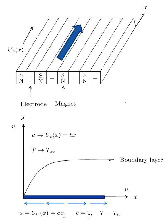
Fig. 1 (a) Structure of Riga plate. (b) Geometry of flow problem. |
Two-dimensional velocity and temperature fields are defined by
$ { V}=[ u( x,y) ,v( x,y) ,0] \,, T=T(x,y)\,. $
The mathematical expression describing the non-Fourier concept is
$ { q}+\delta _{ E}( { V}\cdot { \nabla}{ q}+( { \nabla} \cdot{ V} ) { q}-{ q}\cdot{ \nabla}{ V}) =-k{ \nabla }T\,, $
the above expression for incompressible fluid takes the form
$ { q}+\delta _{ E}( { V}\cdot{ \nabla}{ q}-{ q}\cdot{ \nabla} V) =-k{ \nabla }T\,. $
In above expression $\delta _{ E}$ denotes the thermal relaxation time, $\% { q}$ represents the heat flux, ${ V}$ denotes the fluid velocity, $k$ denotes thermal conductivity, and $T$ represents fluid's temperature.
The governing equations of continuity, momentum and temperature after applying boundary layer approximation are given as the following,
$$ \frac{\partial u}{\partial x}+\frac{\partial v}{\partial y}=0\,, (5) $$
$$ u\frac{\partial u}{\partial x}+v\frac{\partial u}{\partial y}=U_{e}\frac{\% d U_{e}}{d x}+\upsilon \frac{\partial ^{2}u}{\partial y^{2}}+\frac{\pi j_{0}M}{\% 8\rho }\exp \Big( \frac{-\pi }{a_{1}}y\Big) \,, (6) $$
$$ u\frac{\partial T}{\partial x}+v\frac{\partial T}{\partial y}+\delta _{ E}\Omega _{E}=\frac{k}{\rho C_{p}}\frac{\partial ^{2}T}{\partial y^{2}}+\% \frac{\mu }{\rho C_{p}}\Big( \frac{\partial u}{\partial y}\Big) ^{2}\,. (7) $$
Here $u$ and $v$ are the velocity components along axes $x$ and $y$ respectively, $U_{e}$ denotes free stream velocity, $\nu $ is kinematic viscosity, $a_{1}$ is the width for electrodes and magnets, $j_{0}$ expresses the applied current density in electrodes, $M\;(=M_{0}x$) is permanent variable magnets magnetization, $\rho $ depicts fluid density, $T$ denotes fluid's temperature, $k$ represents thermal conductivity, $C_{p}$ is specific heat, absolute viscosity is represented by $\mu $ and $\delta _{ E}$ is thermal relaxation time.
In the above expression, the value of $\Omega _{E}$ is examined as
$ \Omega _{E} = u\frac{\partial u}{\partial x}\frac{\partial T}{\partial x}+v \frac{\partial v}{\partial y}\frac{\partial T}{\partial y}+u\frac{\partial v }{\partial x}\frac{\partial T}{\partial y}+v\frac{\partial u}{\partial y} \frac{\partial T}{\partial x} \\\ +2uv\frac{\partial ^{2}T}{\partial x\partial y} +u^{2}\frac{\partial ^{2}T}{\partial x^{2}}+v^{2}\frac{\partial ^{2}T}{ \partial y^{2}} \\\ -\frac{\mu }{\rho C_{p}}\Big( 2u\frac{\partial u}{\partial y}\frac{ \partial ^{2}u}{\partial x\partial y}+2v\frac{\partial u}{\partial y}\frac{ \partial ^{2}u}{\partial y^{2}}\Big) \,, $
2.1 Boundary Conditions
$$ u=U_{w}( x) =ax\,, \ \ v=0\,, \ \ T=T_{w}\,,\ \ \ \ {\rm at} \ \ y=0\,, u\rightarrow U_{e}( x) =bx\,, \quad T\rightarrow T_{\infty } \ \ \text{when} \ \ y\rightarrow \infty \,, (9) $$
$U_{w}$ is stretching velocity in $x$ direction, $U_{e}$ is ambient or free stream velocity, $a$, $b$ are dimensional constants, $T_{\infty }$ is the ambient fluid temperature, $T_{w}$ is constant wall temperature.
2.2 Transformation
By the induction of suitable variables given below
$ \eta =y\sqrt{\frac{a}{\upsilon }}\,, \ \ u=axf'(\eta )\,, \ \ v=-\sqrt{a\nu }f(\eta )\,, \theta ( \xi ) =\frac{T-T_{\infty }}{T_{w}-T_{\infty }}\,, $
mass conservation law is satisfied identically, however other conservation laws are simplified as follows:
$ f^{\prime \prime \prime }+ff^{\prime \prime }-(f^{\prime })^{2}+S^{2}+Q\exp ( -B\eta ) =0\,, $
$ \theta ^{\prime \prime }+Pr f\theta ^{\prime }+Pr Ec(f^{\prime \prime })^{2}-Pr \gamma ( ff^{\prime }\theta ^{\prime }+( f) ^{2}\theta ^{\prime \prime }) \quad +2Pr \gamma Ec( f^{\prime }(f^{\% \prime \prime })^{2}-ff^{\prime \prime }f^{\prime \prime \prime }) =0\,, $
with boundary conditions:
$ f(0)=0\,, \quad f^{\prime }(0)=1\,, \quad f^{\prime }(\infty )\rightarrow S\,, \\ \theta (0)=1\,, \quad \theta (\infty )\rightarrow 0\,, $
where $S$ represents ratio of rates, $Q$ denotes the modified Hartmann number, $B$ denotes the non-dimensional parameter, $Pr $ shows Prandtl number, $\gamma $ depicts thermal relaxation parameter and $Ec$ denotes Eckert number. In mathematical form these parameters are:
$$ S =\frac{b}{a}\,, \quad Q=\frac{\pi j_{0}M_{0}}{8\rho a^{2}}\,,\quad B=\frac{\pi }{a_{1}}\sqrt{\frac{\upsilon }{a}}\,, Pr =\frac{\mu C_{p}}{k}\,, \quad Ec=\frac{U_{w}^{2}}{C_{p}( T_{w}-T_{\infty }) } \,,\quad \gamma =a\delta _{ E}\,, (14) $$
coefficients of skin friction i.e., $C_{f_{x}}$ is
$ C_{f_{x}}=\frac{{ \tau }_{yx}}{\rho U_{w}^{2}}\,. $
The wall shear stress is given by
$ { \tau }_{yx}=\mu \Big( \frac{\partial u}{\partial y}\Big) _{y=0}\,. $
In dimensionless variables one has
$ C_{f_{x}}{Re}_{x}^{1/2}=f^{\prime \prime }(0)\,, $
where ${Re}_{x}={U_{w}x}/{\upsilon }$ depicts the local Reynolds number.
3 Homotopic Technique
Homotopic technique is developed in 1992 by Liao,[23] which is helpful for the solution construction of highly nonlinear systems. Homotopy is a continuous variation or deformation of an equation or function. It has some advantanges in comparison to other methods i.e., (i) it does not depend on any large or small values selection of emerging parameters (ii) ensure the convergence of series solution (iii) free selection of linear operator and base function. For the computation of homotopic solutions, it is essential to define initial guesses and linear operators which are
$ f_{0}( \eta ) =S\eta +( 1-S) (1-\exp (-\eta ))\,, \ \ \theta _{0}( \eta ) =\exp (-\eta )\,, $
$ \mathcal{L}_{f}( f) =\frac{d^{3}f}{d\eta ^{3}}-\frac{d f}{d\eta }\,, \quad \mathcal{L}_{\theta }( \theta ) =\frac{d^{2}\theta }{d\eta ^{2}}\% -\theta \,, $
with the properties
$ \mathcal{L}f[ B_{1}\exp (-\eta )+B_{2}\exp (\eta )+B_{3}] =0\,, $
$ \mathcal{L}_{\theta }[ B4\exp (-\eta )+B5\exp (\eta )] =0\,. $
It should be noted that $B_{i}$ $( i=1,2,3,\ldots,5) $ represents arbitrary constants.
3.1 Zeroth-Order Problems
$$ ( 1-q) \mathcal{L}f[ \tilde{f}( \eta ;q) -f_{0}( \eta ) ] =q\hbar f\mathcal{N}_{f}[ \tilde{f }( \eta ;q) ,\tilde{\theta }( \eta ;q) ] \,, (22) $$
$$ ( 1-q) \mathcal{L}_{\theta }[ \tilde{\theta }( \eta ;q) -\theta _{0}( \eta ) ] =q\hbar _{\theta }\mathcal{\% N}_{\theta }[ \tilde{f}( \eta ;q) ,\tilde{\theta }\% ( \eta ;q) ] \,, (23) $$
$$ \tilde{f}( 0;q) =0\, \quad \tilde{f}^{\prime }( 0;q) =1\,, \quad \tilde{f}^{\prime }( \infty ;q) =S\,, (24) $$
$$ \tilde{\theta }( 0;q) =1\,,\quad \tilde{\theta }\% ( \infty ;q) =0\,, (25) $$
$ \mathcal{N}_{f}[ \tilde{f}( \eta ,q) ] = \frac{\% \partial ^{3}\tilde{f}( \eta ;q) }{\partial \eta ^{3}}+\% \tilde{f}( \eta ;q) \frac{\partial ^{2}\tilde{f}( \eta ;q) }{\partial \eta ^{2}}-\Big( \frac{\partial \tilde{f}\% ( \eta ;q) }{\partial \eta }\Big) ^{2} +S^{2}+Q\exp ( -B\eta ) \,, $
$ \mathcal{N}_{\theta }[ \tilde{\theta }( \eta ;q) ] = \frac{\partial ^{2}\tilde{\theta }( \eta ;q) }{\partial \eta ^{2}}+Pr \tilde{f}( \eta ;q) \frac{\partial \tilde{\% \theta }(\eta ,q)}{\partial \eta }+Pr Ec\Big( \frac{\partial ^{2}\% \tilde{f}( \eta ;q) }{\partial \eta ^{2}}\Big) ^{2} -Pr \gamma \Big( \tilde{f}( \eta ;q) \frac{\partial \tilde{f}( \eta ;q) }{\partial \eta }\frac{\partial \tilde{\theta }(\eta ,q)}{\partial \eta }+( \tilde{f}( \eta ;q) ) ^{2}\Big) +2Pr \gamma Ec\Big( \frac{\partial \tilde{f}( \eta ;q) }{\% \partial \eta }\Big( \frac{\partial ^{2}\tilde{f}( \eta ;q) }{\partial \eta ^{2}}\Big) ^{2}-\tilde{f}( \eta ;q) \frac{\% \partial ^{2}\tilde{f}( \eta ;q) }{\partial \eta ^{2}}\frac{\% \partial 3\tilde{f}( \eta ;q) }{\partial \eta ^{3}}\Big)\, . $
$q$ represents embedded parameter and varies from zero to one and non-zero auxiliary parameters are $\hbar _{f}$ and $h_{\theta }$
3.2 $k$-th Order Deformation Problems
$ \mathcal{L}_{f}[ f_{k}( \eta ) -\chi _{k}\% f_{k-1}( \eta ) ] =\hbar _{f}\mathcal{R}_{k}^{f}( \eta ) \,, $
$ \mathcal{L}\theta [ \theta _{k}( \eta ) -\chi _{k\% }\theta _{k-1}( \eta ) ] =\hbar _{\theta }\mathcal{R}\% _{k}^{\theta }( \eta ) \,, $
$ f_{k}( 0) =0\,,\quad f_{k}^{\prime }( 0) =0\,, \quad \ f_{k}^{\prime }( \infty ) =0\,, $
$ \theta _{k}( 0) =0\,,\quad \theta _{k}( \infty ) =0\,. $
For $k$-th order:
$ \mathcal{R}_{k}^{f}( \eta ) =f_{k-1}^{\prime \prime \prime }+\sum_{p=0}^{k-1}( f_{k-1-p}f_{p}^{\prime \prime }) -\sum_{p=0}^{k-1}( f_{k-1-p}^{\prime }f_{p}^{\% \prime }) +S^{2}( 1-\chi _{k}) +Q\exp ( -B\eta ) \,, $
$ \mathcal{R}_{k}^{\theta }( \eta ) =\theta _{k-1}^{\prime \prime } +Pr \sum_{p=0}^{k-1}( f_{k-1-p}\theta _{p}^{\prime }) +Pr Ec\sum_{p=0}^{k-1}( f_{k-1-p}^{\prime \prime }f_{p}^{\% \prime \prime }) -Pr \gamma \Big( \sum_{p=0}^{k-1}f_{k-1-p}\sum_{m=0}^{p}( f_{p-m}^{\% \prime }\theta _{m}^{\prime }) +\sum_{p=0}^{k-1}f_{k-1-p}\sum_{m=0}^{p}( f_{p-m}^{}\theta _{m}^{\prime \prime }) \Big) +2Pr \gamma Ec\Big( \sum_{p=0}^{k-1}f_{k-1-p}^{\prime }\sum_{m=0}^{p}( f_{p-m}^{\prime \prime }f_{m}^{\% \prime \prime }) +\sum_{p=0}^{k-1}f_{k-1-p}\sum_{m=0}^{p}( f_{p-m}^{\prime \prime }f_{m}^{\prime \prime \prime }) \Big) \,. $
Obviously for $q=0$ and $q=1$, one may write%
$$ \tilde{f}( \eta ;0) =f_{0}( \eta ) \,, \quad \tilde{f}( \eta ;1) =f( \eta ) \,, \tilde{\theta }( \eta ;0) =\theta _{0}( \eta ) \,, \quad \tilde{\theta }( \eta ;1) =\theta ( \eta )\, , $$
and with variation of $q$ from $0$ to $1$, $\tilde{f}( \eta ;q) $ and $\tilde{\theta }( \eta ;q) $ vary from the initial solutions $f_{0}( \eta ) $ and $\theta _{0}(\eta )$ to the final solutions $f( \eta ) $ and $\theta (\eta )$ respectively. Using Taylor series for $q=1$, we have
$ f( \eta ) =f_{0}( \eta ) +\sum_{k=1}^{\infty }f_{k}( \eta ) \,, $
$ \theta ( \eta ) =\theta _{0}( \eta ) +\sum_{k=1}^{\infty }\theta _{k}( \eta ) \,. $
The general solutions $( f_{k} \text{ and }\theta _{k}) $ of Eqs. (29)--(32) corresponding to special solutions $( f_{k}^{\% \ast }\text{ and }\theta _{k}^{\ast }) $ are
$ f_{k}( \eta ) =f_{k}^{\star }( \eta ) +B_{1}e^{-\eta }+B_{2}e^{\eta }+B_{3}\,, $
$ \theta _{k}( \eta ) =\theta _{k}^{\star }( \eta ) +B_{4}e^{-\eta }+B_{5}e^{\eta }\,, $
where the constants $B_{i}$ $(i=1,2,\ldots,5)$ are computed through the boundary conditions (33). We ultimate have
$ B_{2} =0\,,\quad B_{1}=-\frac{\partial f_{k}^{\star }( \eta ) }{\partial \eta }\Bigm| _{\eta =0}\,, \\ B_3=-f_{k}^{\star }( 0) - \frac{\partial f_{k}^{\% \star }( \eta ) }{\partial \eta }\Bigm| _{\eta =0}\,, \\ B_{5} =0\,, \quad B_{4}=-\theta _{k}^{\star }( 0)\,. $
4 Convergence of the Series Solutions
Homotopic technique provides and guarantees the convergent series solutions in an easy way. To ensure the convergence graphical behavior of solutions are constructed corresponding to auxiliary parameters (see Fig. 2). This figure witnesses that the acceptable convergence regions are $-1.7\leq \hbar _{f}\leq -0.3$ and $-1.8\leq \hbar _{\theta }\leq -0.4$.

Fig. 2 $h$-curves for $f(\eta )$ and $\theta (\eta )$. |
5 Disscusion
This section reports that how representative physical parameters affect various quantities of interest such as velocity and temperature distributions. For this purpose, Figs. 3--9 are displayed. Figure 3 depicts the velocity field, $f^{\prime }(\eta )$ is sketched against ration parameter $S$. It is identified that velocity field rises with increasing ration parameter $S$. Its boundary layer thickness gets steeper with increasing $S$. Physically increasing values of ration parameter $S$ induces a supporting free stream velocity, which helps enhancing the velocity distribution.
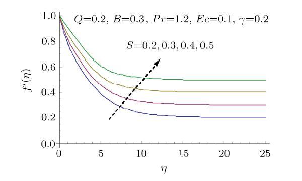
Fig. 3 Effect of $S$ on $f^{\prime }$. |
Figure 4 illustrates the velocity distribution corresponding to modified Hartmann number $Q$. Higher intensity of modified Hartmann number $Q $ give rise to velocity distribution. Physically modified Hartman number $Q $ is dominating and thus it assists the flow due to more intensity of external electric field and as a consequence the wall parallel lorentz force produces. Hence the velocity field exceeds. Moreover the thicker velocity boundary layer is observed corresponding to growing $Q$. Figure 5 demonstrates how the Prandtl number $Pr$ affects the temperature distribution. An expecting observation is made from this figure i.e. temperature decays with increasing Prandtl number $Pr$. For larger Prandtl number $Pr$ the momentum diffusivity effects dominate the effect of thermal diffusivity, which shifts the low transfer of heat from heated surface towards the cold ambient fluid. As a consequence the temperature reduces. Figure 5 further shows that thermal boundary layer becomes thinner with growing $Pr$. Figure 6 is plotted to see the behavior of temperature distribution against dimensionless Eckert number $Ec$. This figure illustrates the increasing trend of temperature field for dominating effects of Eckert number $Ec$. The variation in fluid temperature is confined to a thick boundary layer. %This makes evident the existance of thick thermal boundary %layer for larger Eckert number $Ec$. However due to dominating Eckert number $Ec$ more heat generation in fluid occurs because of strong friction force between the fluid particles. Therefore fluid temperature rises.
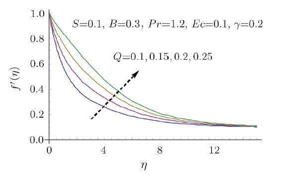
Fig. 4 Effect of $Q$ on $f^{\prime }$. |
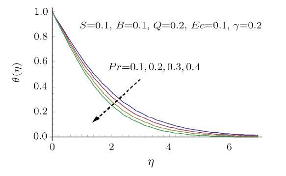
Fig. 5 Effect of $Pr $ on $\theta $. |
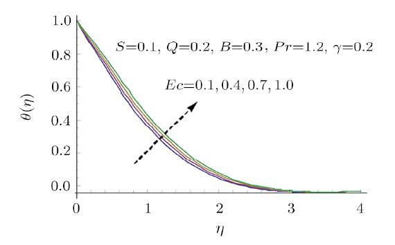
Fig. 6 Effect of $Ec$ on $\theta $. |
Figure 7 shows how the modified Hartman number $Q$ affects the temperature distribution. The temperature decreases with increasing modified Hartman number $Q$. The thick thermal boundary layer can be seen for larger $Q$. The temperature exceeds at the surface of the sheet due to the assistance provided by the wall parallel Lorentz force to the flow induced by stretchable Riga plate. However it gradually decreases away from the surface. Hence the temperature distribution decays. Figure 8 plots the temperature distribution versus thermal time relaxation parameter $\gamma $. The fluid's temperature and the thickness of associated boundary layer decreases with increasing $\gamma $. In fact for larger thermal time relaxation parameter $\gamma $ the fluid particles take additional time for transporting heat to the adjacent particles, which illustrates decrement in temperature field. Fourier model deduces by setting $\gamma =0$. In this case the heat is transferred through out the material with infinite speed and thus temperature distribution raises for $\gamma =0$. Figure 9 discloses the effects of ration parameter $S$ and modified Hartman number $Q$ on skin friction coefficient $Cf$. The skin friction coefficient $Cf$ decreases with increasing ration parameter $S$ and modified Hartman number $Q$. Figure 10 reflects the behavior of streamlines for the present flow.
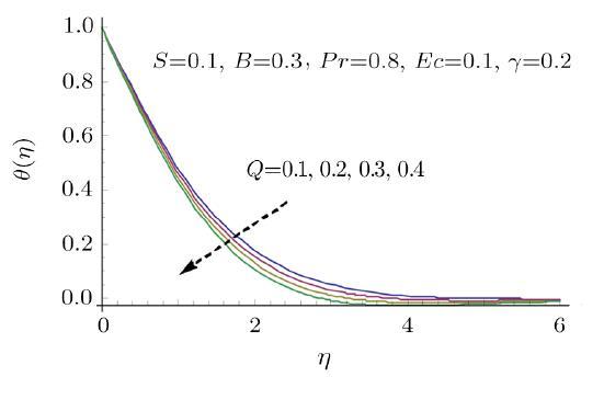
Fig. 7 Effect of $Q$ on $\theta $. |
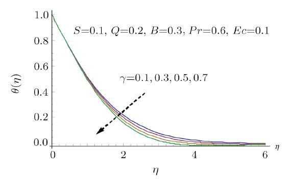
Fig. 8 Effect of $\gamma $ on $\theta $. |
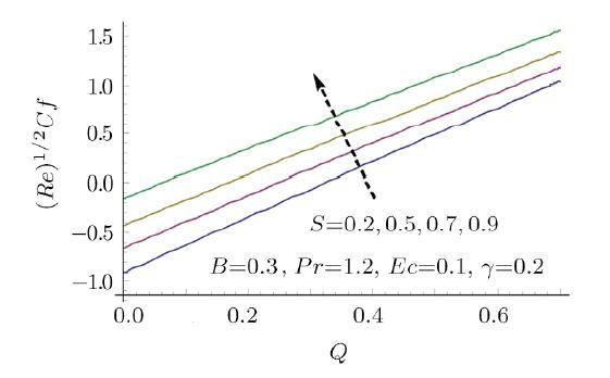
Fig. 9 Effec of $S$ and $Q$ on $Cf$. |

Fig. 10 Streamlines for the flow. |
6 Conclusions
We present the mathematical analysis to explore the heat transfer effects via Cattaneo-Christov heat flux model with viscous dissipation on staganation point flow past a stretchable Riga plate. We obtained the exact expression for velocity and temperature field which is computed analytically. Graphs display how the involved parameters affect the abovementioned distributions. The concluding points in the whole study are listed below:
(i) The flow velocity increases and boundary layer associated with velocity become thick by dominating modified Hartman number $Q$ and ratio parameter $S$.
(ii) Eckert number $Ec$ increases the temperature distribution.
(iii) An increase in modified Hartman number $Q$ leads to decay the fluid's temperature.
(iv) Temperature decreases with increasing thermal relaxation parameter $% \gamma $.
(vi) Skin frictio/drag force can be increased by enhancing $S$ and $Q$.