


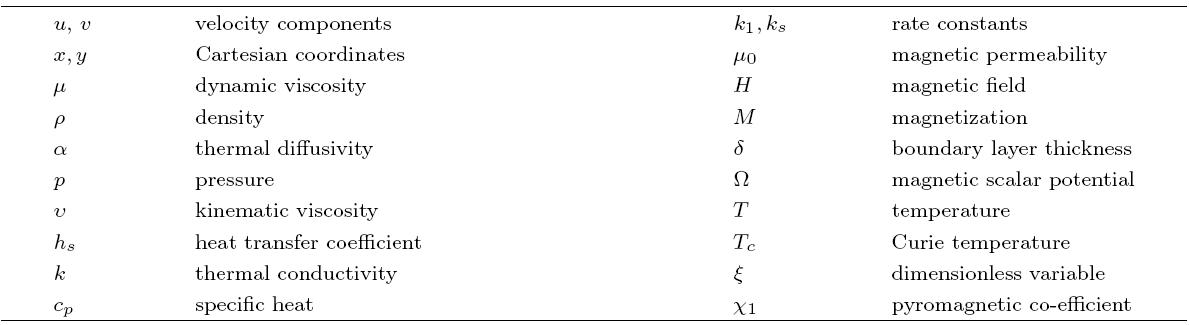
Nomenclature |
 |
1 Introduction
The packed bed tabular reactions of cooled or heated walls are usually employed in industry to accomplish heterogeneous or homogeneous catalytic reactions, which can be endothermic or exothermic. In gas-solid transport-reaction mechanisms, reaction take place within the solid phase, within liquid phase, or at liquid interface. Reaction between atoms/molecules of sundry coefficients can take place during their collision and or a third distinct atom/molecule may be sufficient for a reaction to occur. Several chemical reactions proceed very slowly, on not at all, except in the presence of a catalyst. A survey of the chemical aspects of heterogeneous, or surface reactions have been characterized by Scott,[1] and Gray and Scott.[2] A full talk of catalysis and a description of several of its practical applications is discussed in Refs. [3-5]. A heterogeneous mixture includes of either or both of (i) hydrophilic and hydrophobic materials in a unique mixture, or (ii) sundry conditions of matter; hydrophilic and hydrophobic materials would be a mixture of silicone grease, octane, and water. Fluids, solids, heterogeneous, and gasses might be made homogeneous by mixing, melting, or by permitting time to go for diffusion to appropriate the atoms/molecules equitably. For instance, mixing dye to water will make a heterogeneous solution, however, later on it reduced to a homogeneous. Homogeneous and heterogeneous reactions are important in several chemically reacting procedures. Homogeneous and heterogeneous reactions are important in several chemically reacting procedures. Merkin[6] initiated the chemically reactive species in the flow induced by stretching sheet. The friction drag in a chemically reactive species was scrutinized by Chaudhary and Merkin.[7] Bachok et al.[8] characterized the effects of homogeneous$-$heterogeneous reactions in liquid flow. Kameswaran et al.[9] expressed heat transfer in a chemically reactive species in the flow of a nanofluid. Khan and Pop[10] characterized the two-dimensional flow of a chemically reactive species in the presence of stagnation point.
A liquid that becomes magnetized in the presence of ferrite nanoparticles and an external magnetic field is termed as ferrofluid, initiated by Papell.[11] Water or an organic solvent is usually the carrier liquid. In present analysis, the carrier liquids are taken with three chemical species. Drug targeting is the delivery of medications to organ or receptors or some other particular part of the body to which one wants to deliver the drug. Different nonmagnetic nanocarries (microspheres, microparticles, and nanoparticles and so forth.) are effectively used for drug targeting but they demonstrate poor site specificity and are quickly cleaned up by reticuloendothelial system under ordinary circumstances.[12] Taking into account these reasons, ferromagnetic fluid is studied in the presence of three different chemical species. Thermomagnetization coupling make ferromagnetic liquids and heat transfer in several viscous and non-Newtonian fluids are more valuable in various applications.[13-34]
Merkin[35] specified four common ways through which temperature distribute from wall to ambient fluid, i.e., $(i)$ prescribed surface heat flux distributions, $(ii)$ prescribed wall temperature distributions, $(iii)$ conjugate conditions, and $(iv)$ Newtonian heating. In conjugate condition, heat transfer from a bounding wall of finite heat capacity and thickness. The interface temperature depends on the intrinsic characteristics of the system, i.e., thermal conductivity of solid and liquid. On the other hand, in Newtonian heating, the heat transfer rate from the bounding wall (of finite heat capacity) is proportional to the local surface temperature. It is also known as conjugate convective flow.
Recently, the scientists and researchers are interested to arise the rate of cooling or heating and reduce the friction drag in the advanced technological procedures. Thus different models were constructed for the reduction of drag forces or friction drag, for example, flows over the surface of a tail plane, wing, and wind turbine rotor, etc. However, the friction drag can be decreased by keeping boundary layer away from the separation and keeping the transition of the laminar to turbulent flow delay. This task can be executed through sundry physical features such as fluid suction and injection, through moving the surface, and the presence of different body forces. Similarly, the scientists have developed different types of boundary conditions that are applicable in the enhancement of rate of heating/cooling over the surface. Thus, the aim of the analysis concentrates on the reduction of friction drag and enhancement of rate of heating. A hybrid isothermal model for the ferrohydrodynamic flow in a chemically reactive species is taken in this direction. The hybrid isothermal model for chemically reactive species is an extension of the work of Merkin,[6] in the present model three chemical species are considered. The aim of the present work is that by incorporating three different chemical species will enhance the heat transfer rate in presence of magnetic dipole. Thus in the present work, heat transfer rate and friction drag is evident for the hybrid chemically reactive species. The transport equations are taken by incorporating the boundary layer assumptions. Further, the boundary value problem is solved analytically with the help of BVPh2-mid point method and optimal homotopy analysis method (OHAM). The materialized parameters are described via graphs and tables.
2 Ferrohydrodynamic, Energy, and Concentration Equations
2.1 Flow Analysis
A hybrid model for homogeneous-heterogeneous reactions is considered for the incompressible ferrohydrodynamic boundary layer flow along with the isothermal cubic autocatalytic reactions, given schematically by
$ A+C+C\rightarrow 3C,\text{rate}=k_{1}ac^{2}\,, $
$ B+C+C\rightarrow 3C,\text{rate}=k_{1}bc^{2}\,, $
while the first order, hybrid isothermal reactions on the catalyst surface are
$ A\rightarrow C,\quad{\rm rate}=k_{s}a\,, $
$ B\rightarrow C,\quad{\rm rate}=k_{s}b\,, $
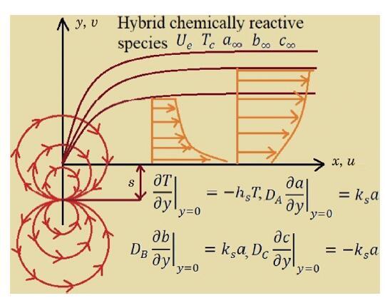
here $a,b,$ and $c$ characterize the concentrations of chemical species A,B, and $C$. It is presumed that the reactants $A$ and $B$ have constant concentration $a_{0}$ and in the external flow there is no autocatalyst $C$. Then the reactions given in Eqs. (1) and (2) confirm that at the outer edge of the boundary layer and in the exterior flow the reaction rate will be zero. The heat release by the reaction is considered negligible. Further, the flow is scrutinized in the presence of a magnetic dipole. The center of magnetic dipole lies on the $y$-axis at a distance $s$ away from the $x$-axis. The physical schematic for the flow inspection is shown in Fig. 1. In present analysis, the fluid is assumed to be heated, i.e., $ T_{w}<T_{\infty } assumed to be heate<T_{c}$. The fluid above $T_{c}$ is not capable of being magnetized. Employing the boundary layer approximation $u=x=O\left( 1\right) $ and $v=y=O\left( \delta \right) $, the ferrohydrodynamic, thermal energy, and concentration boundary layer equations are
$ \qquad \frac{\partial u}{\partial x}+\frac{\partial v}{\partial y}=0\,, $
$ \qquad \rho \left( u\frac{\partial u}{\partial x}+v\frac{\partial u}{\partial y}\% \right) =-\frac{\partial P}{\partial x}+\mu _{0}M\frac{\partial H}{\partial x\% }+\mu \frac{\partial ^{2}u}{\partial y^{2}}\,, $
$ \qquad \rho c_{p}\left( u\frac{\partial T}{\partial x} +v\frac{\partial T}{\partial y }\right) \quad +c_{p}\mu _{0}T\left( u\frac{\partial H}{\partial x} +v\frac{ \partial H}{\partial y}\right) \frac{\partial M}{\partial T} =k\frac{\partial ^{2}T}{\partial y^{2}}\,, $
$ \qquad u\frac{\partial a}{\partial x}+v\frac{\partial a}{\partial y}=D_{A}\frac{\% \partial ^{2}a}{\partial y^{2}}-k_{1}ac^{2}\,, $
$ \qquad u\frac{\partial b}{\partial x}+v\frac{\partial b}{\partial y}=D_{B}\frac{\% \partial ^{2}b}{\partial y^{2}}-k_{1}bc^{2}\,, $
$ \qquad u\frac{\partial c}{\partial x}+v\frac{\partial c}{\partial y}=D_{C}\frac{\% \partial ^{2}c}{\partial y^{2}}+k_{1}ac^{2}+k_{1}bc^{2}\,. $
The permissible boundary conditions are
$ \left. \left. u\right\vert _{y=0}=U_{w}=\frac{u_{0}x}{l}\,,~~\left. v\right\vert _{y=0}=0\,,~~\left. \frac{\partial T}{\partial y} \right\vert _{y=0}=-h_{s}T\,,\right.\nonumber\\ \left. \left. D_{A}\frac{\partial a}{\partial y}\right\vert _{y=0}\!=\!k_{s}a\,,\% \left. D_{B}\frac{\partial b}{\partial y}\right\vert _{y=0}\!=\!k_{s}a\,, \left. D_{C}\frac{\partial c}{\partial y}\right\vert _{y=0}\!=\!-k_{s}a\,,\right. \nonumber\\ \left. \left. u\right\vert _{y\rightarrow \infty }\rightarrow U_{e}=0\,,~~ \left. T\right\vert _{y\rightarrow \infty }\rightarrow T_{\infty }=T_{c}\right.\,, \nonumber\\ \left. \left. a\right\vert _{y\rightarrow \infty }\rightarrow a_{0}\,,~~ \left. b\right\vert _{y\rightarrow \infty }\rightarrow a_{0}\,,~~ \left. c\right\vert _{y\rightarrow \infty }\rightarrow 0\,.\right. $
Here $U_{w}$ exemplifies the characteristic velocity, $l$ signifies the characteristics length, $U_{e}$ identifies velocity of the fluid.
2.2 Magnetic Dipole
The presence of magnetic dipole causes magnetic field, which effects the flow of ferrofluid. The region of the magnetic dipole describes the magnetic scalar potential $\Omega $, which is given below
$ \Omega =\frac{\alpha _{1}}{2\pi }\frac{x}{x^{2}+(y+s)^{2}}\,, $
here $\alpha _{1}$ symbolizes the strength of magnetic field. $H_{x}$ and $% H_{y}$\ signify the components of the magnetic field ($H$)%
$ H_{x}=-\frac{\partial \Omega }{\partial x}=\frac{\alpha _{1}}{2\pi }\frac{\% x^{2}-(y+s)^{2}}{(x^{2}+(y+s)^{2})^{2}}\,, $
$ H_{y}=-\frac{\partial \Omega }{\partial y}=\frac{\alpha _{1}}{2\pi }\frac{\% 2x(y+s)}{\left( x^{2}+(y+s)^{2}\right) ^{2}}\,. $
The magnetic body force for the present case is defined as
$ H=\sqrt{\left( H_{x}\right)^{2}+\left( H_{y}\right) ^{2}}\,. $
Inserting Eqs. ($13$) and ($14$) in Eq. ($15$), we obtain the accompanying Eqs. ($16$) and ($17$), after reached out in powers of $x$ and held terms up to $x$,
$ \frac{\partial H}{\partial x}=-\frac{\alpha _{1}}{2\pi }\frac{2x}{(y+s)^{4}}\,, $
$ \frac{\partial H}{\partial y}=\frac{\alpha _{1}}{2\pi }\left( -\frac{2}{ (y+s)^{3}}+\frac{4x^{2}}{(y+s)^{5}}\right) \,. $
The magnetization $M$ is taken to be a linear function of temperature $T$ as defined below,
$ M=\chi _{1}(T-T_{\infty })\,. $
Figure 1 describes the physical schematic of the ferrofluid.
3 Solution Procedure
Here the dimensionless variables for the present analysis are
$ \quad \psi(\eta,\xi)=\Bigl(\frac{\mu}{\rho}\Bigr)\eta f( \xi ),\quad a=a_{0}g( \xi )\,, \quad b=a_{0}h( \xi )\,, \quad c=a_{0}j( \xi ),\quad \frac{T-T_{c}}{T_{c}}=\theta _{1}( \xi ) +\eta ^{2}\theta _{2}(\xi ) \,, $
here $\theta \left( \xi \right) $\ exhibits dimensionless temperature and $ \mu $\ displays dynamic viscosity, the relating non-dimensional directions are
$ \xi =\frac{y}{l}\sqrt{{Re}},\text{ \ } \eta =\frac{x}{l}\sqrt{{Re}},\text{ \ } {Re}= \frac{u_{0}l}{\upsilon }\,. $
The stream function $\psi \left( \xi \right) $ is defined in such that the equation of mass continuity is identically fulfilled and the velocity components $(u,v)$ are defined as follow
$ u=\frac{\partial \psi }{\partial y}=\frac{u_{0}x}{l}f^{\prime }\left( \xi \right), v=-\frac{\partial \psi }{\partial x}=-\frac{1}{l}\sqrt{\% \frac{u_{0}\mu l}{\rho }}f( \xi ) \,, $
utilizing the similarity variables given in Eqs. (19)--(21), Eqs. (6)--(10) along with boundary conditions given in Eq. (11) take the form of boundary value problem%
$ \qquad f^{\prime \prime \prime }+ff^{\prime \prime }-f^{\prime 2}-\frac{2\beta \theta _{1}}{\left( \xi +\gamma \right) ^{4}}=0\,, $
$ \qquad \theta _{1}^{\prime \prime }+Pr f\theta _{1}^{\prime }+\frac{2\lambda \beta f\left( \theta _{1}-\varepsilon \right) }{\left( \xi +\gamma \right) ^{3}} -4\lambda f^{\prime 2}=0\,, $
$ \theta _{2}^{\prime \prime }-Pr \left( 2f^{\prime }\theta _{2}-f\theta _{2}^{\prime }\right) +\frac{2\lambda \beta f\theta _{2}}{\left( \xi +\gamma \right) ^{3}}-\lambda \beta \theta _{1}- \times\Bigl( \frac{2f^{\prime }}{( \xi +\gamma ) ^{4}}+\frac{4f}{( \xi +\gamma ) ^{5}}\Bigr) -4\lambda f^{\prime \prime 2}=0\,, $
$ \qquad\frac{1}{Sc}g^{\prime \prime }+fg^{\prime }-Kgj^{2}=0\,, $
$ \qquad\frac{\delta _{1}}{Sc}h^{\prime \prime }+fh^{\prime }-Khj^{2}=0\,, $
$ \qquad\frac{\delta _{2}}{Sc}j^{\prime \prime }+fj^{\prime }+Kj^{2}(g+h)=0\,, $
$ \qquad f(\xi )=0, f^{\prime }(\xi)=1, \theta _{1}^{\prime }(\xi )=-\lambda _{1}(1+\theta _{1}(\xi )), \theta _{2}(\xi )=0\,,\quad g^{\prime }(\xi)=K_{s}g(0)\,, \delta _{1}h^{\prime }(\xi )=K_{s}g(0), \delta _{2}j^{\prime }(\xi )-K_{s}g(0)=0, \text{at }\xi =0\,, $
$ f^{\prime }(\xi)\rightarrow 0, \theta _{1}(\xi )\rightarrow 0\,, \theta _{2}(\xi )\rightarrow 0, g(\xi )\rightarrow 1,~~ h(\xi )\rightarrow 1, j(\xi )\rightarrow 0,\text{ when }\xi \rightarrow \infty \,. $
In above boundary value problem, the dimensionless materialized parameters are $\beta $ (ferrohydrodynamic interaction), $K$ and $K_{s}$ (the strengths of the homogeneous and heterogeneous reactions respectively), $\lambda $ (viscous dissipation), $\delta _{c}$ (Curie temperature), $\delta _{1}$ and $ \delta _{2}$ (the ratio of diffusion coefficients), $\lambda _{1}$ (Conjugate parameter due to Newtonian heating), $Sc$ (Schmidt number), $Pr$ (Prandtl number) and $\gamma $ (dimensionless distance). These parameters are described as
$ \qquad \delta _{1}=\frac{D_{B}}{D_{A}}\,,\quad Pr =\frac{\upsilon }{ \alpha }\,,\quad\beta =\frac{\alpha _{1}}{2\pi }\frac{\mu _{0}\chi _{1}T_{c}\rho }{\mu ^{2}}\,, \qquad K_{s}=\frac{k_{s}l}{D_{A}\sqrt{{Re}}} \,,\quad\delta _{c}=\frac{T_{\infty }}{T_{c}}\,, \qquad K=\frac{k_{1}a_{0}^{2}l}{u_{0}}\,,\quad \lambda _{1}=lh_{c}\sqrt{ \frac{\mu }{\rho lu_{0}}}\,,\quad \lambda =\frac{u_{0}\mu ^{2}}{\rho kT_{c}} \,, \qquad \gamma =\sqrt{\frac{u_{0}\rho s^{2}}{\mu }}\,, \quad\delta _{2}= \frac{D_{C}}{D_{A}}\,. $
The chemically reactive species $A,$ $B,$ and $C$ are considered to be of the same size, due to this assumption the diffusions species coefficients $% D_{A},$ $D_{B},$ and $D_{C}$ are equivalent i.e., $\delta _{1}=\delta _{2}=1$, at that point we have
$ g(\xi )+j(\xi )=1,\quad h(\xi )+j(\xi )=1\,. $
Through Eqs. (24)--(26), we obtain the following equation
$ \frac{1}{Sc}g^{\prime \prime }+fg^{\prime }-2Kg\left( 1-g\right) ^{2}=0\,, $
with corresponding boundary conditions are
$ g^{\prime }(\xi )=K_{s}g(\xi ),\text{ at }\xi =0\text{, }g(\xi )\rightarrow 1\text{, as }\xi \rightarrow \infty \,. $
The physical parameters of engineering interest are defined as
$ C_{f}=\frac{2\tau _{w}}{\rho U_{w}^{2}},\text{ }Nu_{x}=\frac{xq_{c}}{\% k\left( T-T_{c}\right) }\,, $
here $\tau _{w}$ (wall shear stress) and the heat flux $q_{c}$ are
$ \tau _{w}=\mu \left. \frac{\partial u}{\partial y}\right\vert _{y=0},\text{ }q_{c}=-\left. k\frac{\partial T}{\partial y}\right\vert _{y=0}\,, $
finally, the dimensionless equations for the friction drag and Nusselt number (the ratio of convective heat transfer coefficient to conductive heat transfer coefficient) i.e. local surface heat flux
$ \frac{{Re}_{x}^{1/2}}{2}C_{f}=f^{\prime \prime }\left( 0\right)\,,\nonumber \\ {Re}_{x}^{\!-\!1/2}Nu_{x}=\!-\!\lambda _{1}\left( 1\!+\!\frac{1}{\theta _{1}(0)\!+\!\eta ^{2}\theta _{2}(0)}\right)\,. $
The boundary value problem is solved by utilizing the optimal HAM and BVPh$ 2$-Midpoint method. The optimal HAM[36-37] is proposed to achieve series solution of highly non-linear differential equations. This technique is free of large/small physical parameters. Besides, optimal HAM is different from all other previous procedures, It gives us with a simple way to control and adjust the convergence of series solution. In the present analysis, optimal HAM is incorporated for the solution of boundary value problem. The corresponding linear operators and initial guesses are
$ L_{f}\left( f\right) =\frac{{\rm d}^{3}f}{{\rm d}\xi ^{3}}+\frac{{\rm d}^{2}f}{{\rm d}\xi ^{2}} ,\quad L_{\theta _{1}}\left( \theta _{1}\right) =\frac{{\rm d}^{2}\theta _{1}}{{\rm d}\xi ^{2}} -\theta _{1}\,, L_{\theta _{2}}\left( \theta _{2}\right) =\frac{{\rm d}^{2}\theta _{2} }{{\rm d}\xi ^{2}}-\theta _{2},\quad L_{g}\left( g\right) =\frac{{\rm d}^{2}g}{{\rm d}\xi ^{2}}-g\,, $
$ f_{0}\left( \xi \right) =1-\exp \left( -\xi \right),\quad \theta _{1_{0}}\left( \xi \right) =\frac{\lambda _{1}}{1-\lambda _{1}}\exp \left( -\xi \right) \,, $
$ \theta _{2_{0}}\left( \xi \right) =0,\quad g_{0}\left( \xi \right) =1-\frac{K_{s}}{ 1+K_{s}}\exp \left( -\xi \right) \,, $
where $f_{0}(\xi ),$ $\theta _{1_{0}}\left( \xi \right) ,\theta _{2_{0}}\left( \xi \right) ,$ and $g_{0}\left( \xi \right) $ signify the initial guesses of $f,\theta _{1},\theta _{2},$ and $g$ respectively, on the other hand $L_{f}\left( f\right) ,$ $L_{\theta _{1}}\left( \theta _{1}\right) ,L_{\theta _{2}}\left( \theta _{2}\right) ,$ and $L_{g}\left( g\right) $ describe the linear operators.
3.1 Convergence Analysis
The physical parameters $\hslash _{f}$, $\hslash _{\theta _{1}},\hslash _{\theta _{2}}$, and $\hslash _{g}$ have leading motivation to control and stabilize the convergence of series solutions. Specified values are assigned to the auxiliary parameters for getting the convergence. In this direction, residual errors are obtained for momentum, energy and concentration equations by defining the equations given below,
$ \Delta _{m}^{f}=\int_{0}^{1}[\mathcal{R}_{m}^{f}( \xi ,\hslash _{f}) ]^{2}{\rm d}\xi \,, $
$ \Delta _{m}^{\theta _{1}}=\int_{0}^{1}[\mathcal{R}_{m}^{\theta _{1}}( \xi ,\hslash _{\theta _{1}}) ]^{2}{\rm d}\xi \,, $
$ \Delta _{m}^{\theta _{2}}=\int_{0}^{1}[\mathcal{R}_{m}^{\theta _{2}}( \xi ,\hslash _{\theta _{2}}) ]^{2}{\rm d}\xi \,, $
$ \Delta _{m}^{g}=\int_{0}^{1}[\mathcal{R}_{m}^{g}( \xi ,\hslash _{g}) ]^{2}{\rm d}\xi \,. $
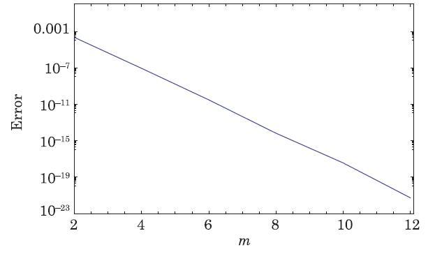
The convergence is displayed by optimal HAM, listed in Tables 1 and 2, using the values of the parameters $\beta =1.2,$ $K=0.8,$ $\lambda _{1}=0.5,$ $K_{s}=1.0,$ $Sc=1.2,$ $Pr =2.0,$ and $\gamma =0.1$. The graphical representation for the $10^{\rm th}$ order approximation display the error decay in Fig. 2.
Table 1 Average residual square errors ($\Delta _{m}^{t}$). |
 |
Table 2 Individual residual square errors for $\Delta _{m}^{f},\Delta _{m}^{\theta _{1}},\Delta _{m}^{\theta _{2}}$, and $\Delta _{m}^{g}$. |
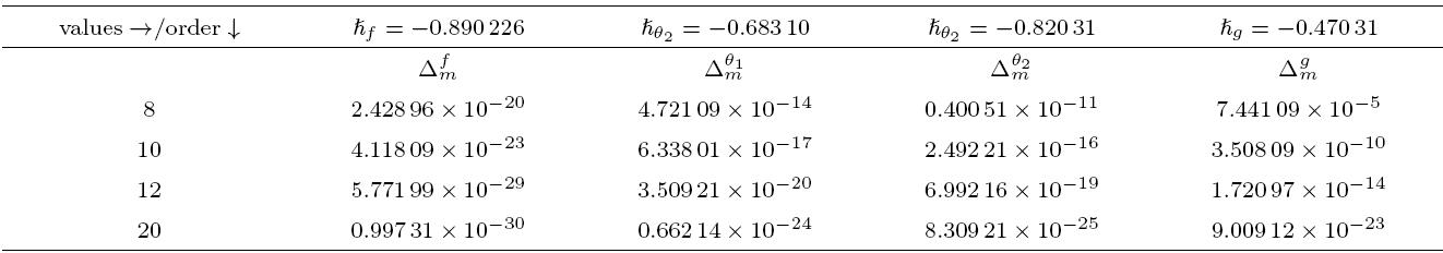 |
Here $\Delta _{m}^{t}$ indicates the total discrete squared residual error.
$ \Delta _{m}^{t}=\Delta _{m}^{f}+\Delta _{m}^{\theta _{1}}+\Delta _{m}^{\theta _{2}}+\Delta _{m}^{g}. $
Here the $\Delta _{m}^{t}$ is used to obtain the optimal convergence control parameters.
4 Results and Discussion
This section concerns the interpretation of sundry materialized parameter on the hybrid chemically reactive species in the viscous ferromagnetic fluid. The characteristics of physical parameters $\lambda _{1}$ (Conjugate parameter due to Newtonian heating), $\beta $ (ferrohydrodynamic interaction), $K$ and $K_{s}$ (the strengths of the homogeneous and heterogeneous reactions respectively), $\lambda $ (viscous dissipation), $Sc$ (Schmidt number), $\delta _{c}$ (Curie temperature), $Pr $ (Prandtl number), and $\gamma $ (dimensionless distance from origin to center of magnetic dipole) are on the hybrid chemically reactive species in the presence of a magnetic dipole are incorporated. The boundary value problem is analyzed via BVPh2-Midpoint method and optimal homotopy analysis method (OHAM).
The effect of parameter $\lambda _{1}$ (conjugate parameter due to Newtonian heating) on axial velocity and temperature field are exhibited in Figs. 3 and 4. It is portrayed from Fig. 3 that $\lambda _{1}$ (conjugate parameter due to Newtonian heating) decline the axial velocity of fluid. An increase in $\lambda _{1}$ leads to enhance the heat transfer coefficient, as a result, the resistance between fluid layers enhances, which is responsible for the reduction in axial velocity. The influence of parameter $\lambda _{1}$ (conjugate parameter due to Newtonian heating) on temperature field is depicted in Fig. 4. It is obvious that the temperature field of the hybrid chemically reactive species shows increasing impact by increasing the parameter $\lambda _{1}$. The physical interpretation is that, an increment in $\lambda _{1}$ leads to rise the heat transfer coefficient $h_{s}$, as a result, the temperature field enhances. Further, the characteristics of $\lambda _{1}$ (conjugate parameter due to Newtonian heating) on concentration field is evident in Fig. 5. It seems from Fig. 5 that concentration field declines for larger valves of $\lambda _{1}$. In fact, an increase in conjugate parameter leads to decelerate the rate of diffusion of hybrid chemical species, as a result, the concentration field reduces thereby enhancing the thickness of concentration boundary layer evident in Fig. 5.
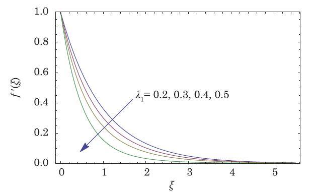
Fig. 3 The effect of parameter $\lambda _{1}$ (conjugate) on axial velocity. |
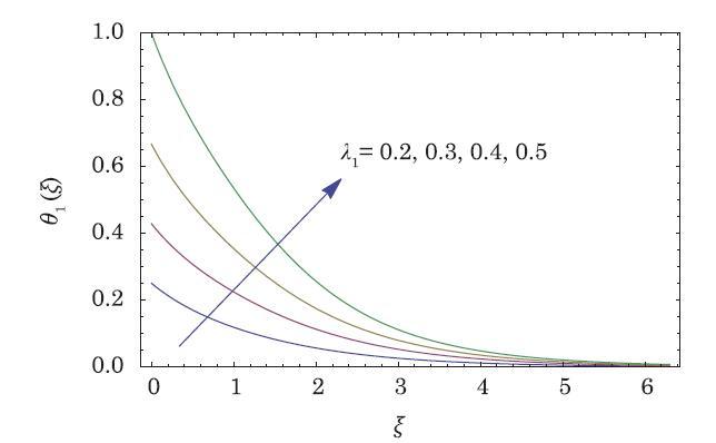
Fig. 4 The effect of parameter $\lambda _{1}$ (conjugate) on temperature field. |
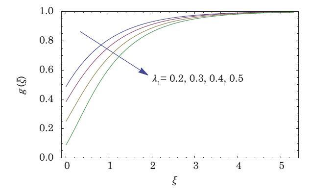
Fig. 5 The effect of parameter $\lambda _{1}$ (conjugate) on concentration field. |
The presence of parameters $\beta $ (ferrohydrodynamic interaction), $% \gamma _{1}$ (dimensionless distance from origin to center of magnetic dipole), and $\varepsilon $ (Curie temperature) assure the characteristic of magnetic dipole on the hybrid chemically reactive species. Figures 6-8 designate the characteristics of ferrohydrodynamic interaction parameter on the axial velocity and temperature field. The axial velocity of hybrid chemically reactive species decline for ferrohydrodynamic parameter evident in Fig. 6. As $\beta $ has a direct relation with viscosity in a linear way, thus by enhancing $\beta $ the hybrid chemically reactive species become more viscous, as a result, the velocity field reduces. Further, the enhancement in viscosity leads to arise friciton between fluid layers, such enhancement in friction is responsible for the increment in temperature field evident in Fig. 7. On the other hand, ferrohydrodynamic parameter declines the concentration profile depicted in Fig. 8. The physical interpretation is that an increment in $\beta $ results in the enhancement of viscosity of the hybrid chemically reactive species, the friction between fluid layers arises, as a result the diffusion of the chemical species reduces.
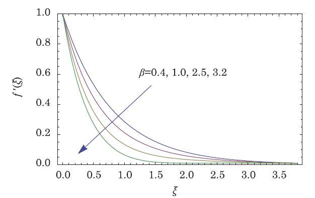
Fig. 6 The effect of parameter $\beta $ (ferrohydrodynamic interaction) on axial velocity. |
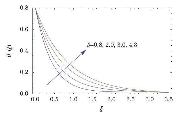
Fig. 7 The effect of parameter $\beta $ (ferrohydrodynamic interaction) on temperature field. |
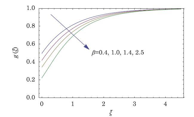
Fig. 8 The effect of parameter $\beta$ (ferrohydrodynamic interaction) on concentration field. |
The characteristics of parameters $K$ (strength of homogeneous reaction), $% Sc $ (Schmidt number), and $K_{s}$ (strength of heterogeneous reaction) on the concentration field are dig out in Figs. 9-11. The influence of $K$ (strength of homogeneous reaction) on the concentration field is evident in Fig. 9. Higher values of $K$ (strength of homogeneous reaction) results in the reduction of concentration field. Whereas, larger values of $% K_{s}$ (strength of heterogeneous reaction) decline the concentration field evident in Fig. 1. The concentration boundary layer thickness arises for higher values of $K$ and $K_{s}$. The physical interpretation is that an enhancement in $K$ and $K_{s}$ leads\linebreak to reduce the diffusion coefficients of hybrid chemically reactive species, as a result, the concentration field reduces, whereas, there concentration boundary layer thickness enhances. The impacts of $Sc$ (Schmidt number) on concentration profile is characterized in Fig. 11.
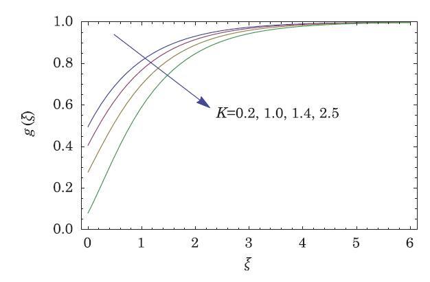
Fig. 9 Effect of $K$ (the strength of homogeneous reaction) on $g(\xi )$. |

Fig. 10 Effect of $K_{s}$ (the strength of heterogeneous reaction) on $% g\left( \xi \right) $. |
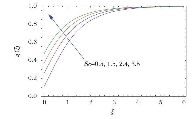
Fig. 11 Influence of $Sc$ (Schmidt number) on concentration field $% g\left( \xi \right)$. |
The higher values of $Sc$ (Schmidt number) improve the concentration field exhibited in Fig. 11, whereas, the concentration boundary layer declines for $Sc$ (Schmidt number). Physically, as $Sc$ (Schmidt number) is proportional to the ratio of momentum diffusivity to mass diffusivity in a linear way, thus $Sc>1.0$ means that momentum diffusivity is greater than mass diffusivity, $Sc=1.0$ means that momentum diffusivity is equal to mass diffusivity, and $Sc<1.0$ means that mass diffusivity is greater than momentum diffusivity. In all these mentioned cases the concentration field arises whereas, the concentration boundary layer thickness reduces.
The influence of Curie temperature on the concentration field is evident in Fig. 12. The temperature field and its corresponding thermal boundary layer thickness arise for Curie temperature $\delta _{c}$ portrayed in Fig. 12. Larger values of Curie temperature lead to higher ambient temperature, as a result the temperature field enhances. The values assigned to remaining parameters are $K=0.8,$ $K_{s}=1.0,$ $\lambda _{1}=0.3,$ $% Sc=1.2,$ $\gamma =0.1,$ and $Pr =2.0$.
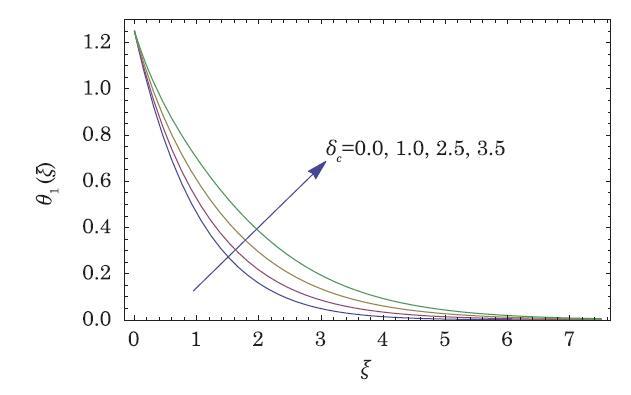
Fig. 12 Impact of $\delta _{c}$ (Curie temperature) on temperature field. |
4.1 Physical Parameters of Engineering Interest
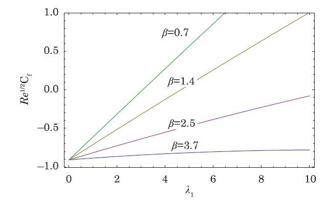
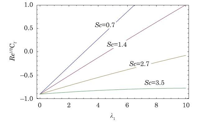
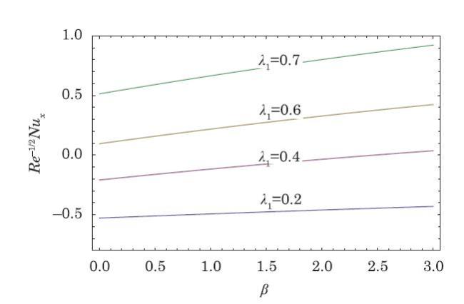
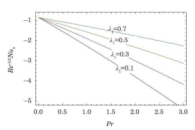
This section concerns the results of physical parameters of engineering interest. These materialized parameters are given in Eqs. (33)-(35). The aim of this section is to scrutinize the impacts of three different chemical species on the rate of heat transfer and friction drag, which are useful in the advanced technological processes. The friction drag via $\lambda _{1}$ (conjugate parameter due to Newtonian heating) for different values $\beta $% (ferrohydodynamic parameter) are portrayed in Fig. 13. It is observed that the ferrohydrodynamic interaction parameter enhance the friction drag of the hybrid chemically reactive species. On the other hand, the friction drag declines for the $Sc$ (Schmidt number) shown in Fig. 14. Further, the impacts of conjugate parameter $\lambda _{1}$ on the heat transfer rate via $% \beta $ (ferrohydrodynamic) in the flow of a hybrid chemically reactive species is depicted in Fig. 15. It is characterized that heat transfer rate enhances for conjugate parameter $\lambda _{1}$. Whereas, an enhancement in heat transfer rate via $Pr $ (Prandtl number) for different values of conjugate parameter $\lambda _{1}$ is designated in Fig. 16. The physical parameters of engineering interest and its impacts on the present flow problem are depicted in Tables 3 and 4.
Table 3 Comparison of Nusselt number for the case when $\beta =1.5,K=0.8,K_{s}=1.2,\lambda _{1}=0.3$. |
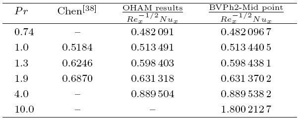 |
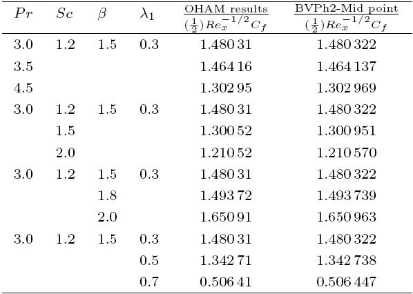
Table 4 The skin friction coefficient $(1/ 2){Re}^{1/2}C_{f}$ for different values of $Pr ,$ $\beta $, $Sc$ and $\lambda _{1}$ are classified and compared by means of analytic solution based on optimal HAM and BVPh2-mid point method. |
 |
5 Concluding Remarks
The present work concentrates on the heat transfer rate and friction drag in a hybrid chemically reactive species. The analysis is carried out for three different chemical species. Mass flux is evaluated by Fick's law. The phenomena of Newtonian heating and magnetic dipole are further considered. The main points of the analysis are as the following.
(i) The conjugate parameter enhances the temperature field thereby declines the axial velocity and concentration field.
(ii) The axial velocity and concentration field of hybrid chemically reactive species decline for ferrohydrodynamic parameter, thereby enhances the temperature filed.
(iii) The strength of homogeneous reaction $K$ results in the reduction of concentration field.
(iv) The strength of heterogeneous reaction $K_{s}$ declines the concentration field.
(v) The Schmidt number $Sc$ improves the concentration field.
(vi) The friction drag via conjugate parameter $\lambda _{1}$ are depicted.
(vii) The heat transfer rate via ferrohydrodynamic and Prandtl number are scrutinized.
Acknowledgment
The authors, therefore, acknowledge technical and financial support of the Higher Education Commission (HEC).