


Nomenclature |
 |
1 Introduction
Study of peristaltic pumping of fluids has been the point of interest and motivation for researchers through many years. Peristalsis in practice is to push the material inside the tube-like structures when the progressive waves of area contraction and expansion are made to propagate along the tube's length. A wide range of applications of peristalsis is reported in medical and engineering science such as in physiology, the mechanism is used by the body to mix and drive the content inside the tube such as urine is pushed from kidney to bladder in ureter duct,[1] digestive system,[2] blood circulation in vessels, bile movement in a bile ducts, movement of food bolus, transport of ovum and cilia are a few applications. Similarly, the working of biomedical instruments such as a heart-lung machine (HLM) and blood pumps used in dialysis are also based on this principle. The same mechanism is also exploited in many industrial processes such as corrosive and toxic fluids are transported through roller and finger pumps.
Mathematical modeling and analysis of peristaltic transport were developed by Shapiro et al.[3] in wave frame and Fung and Yih[4] in the laboratory frame for the Newtonian fluids. Two-dimensional peristaltic means of transport was investigated numerically by Takabatake et al.[5] and Brown et al.[6] without using assumptions of long wavelength and low Reynolds number. Interaction of peristaltic transport and heat transfer has also acquired much attention due to their extensive use in industrial and clinical processes. Laser therapy, cryosurgery, oxygenation and hemodialysis require thermal modeling. Also, other processes like condensation, crystallization, evaporation are amongst the core applications of heat transfer. Radhakrishnamacharya and Srinivasulu[7] studied the peristaltic flow of viscous fluid in presence of wall properties and heat transfer. Mekheimer[8] combined the effects of MHD and heat transfer on wavy motion of viscous fluid in the vertical channel. Srinivas and Kothandapani[9] studied heat effects on the peristaltic motion of fluid through the asymmetric channel. Very recently, Mosayebidorcheh and Hatami[10-11] analytically investigated the heat transfer effects on the peristaltic flow of nanofluids in an asymmetric channel. Bhatti et al.[12] studied the peristaltic transport of two-phase fluid flow with heat and mass transfer in a porous channel.
Magnetohydrodynamics (MHD) refers to study the effects of the magnetic field when applied to the electrically conducting fluids in motion. MHD peristaltic motion fluids are of great importance because of its wide range of applications in geophysics, astrophysics, sensors, engineering and magnetic drug targeting in clinical science. Misra et al.[13] combined heat and MHD effects on the peristaltic motion of a fluid with varying physical and thermal properties in an asymmetric channel. Noreen and Saleem[14] studied MHD peristaltic motion in a porous medium under the Soret and Dufour effects with chemical reaction and thermal radiation. Reddy[15] analytically investigated the velocity slip and MHD effects on the peristaltic flow through a porous medium together with heat and mass transfer. Sud et al.[16] observed the effect of magnetic field on the blood flow and concluded that it increases the velocity of the blood. Akbar[17] investigated the MHD effects with nanoparticles on Eyring-Powell fluid model in peristaltic motion. Agrawal and Anwaruddin[18] studied different aspects of MHD blood flowing peristaltically in the equally branched channel, viewing its applications in cardiac operations and arterial stenosis. Abbasi et al.[19] also analyzed mathematically the effects of variable viscosity on peristaltic motion of MHD fluids with Soret and Dufour relations. Reddy et al.[20-21] conducted the study of peristaltic flow of an incompressible non-Newtonian fluid in presence of MHD and partial slip effects in asymmetric channel.
Influence of Joule heating on peristaltic flow of fluidswith constant electrical conductivity has been carried out by many researchers, such as Refs.[22-24] but none has related temperature dependent electrical conductivity with peristalsis as per authors' knowledge. In this paper, we propose a peristaltic flow model of Newtonian fluid with variable electrical conductivity. Assumptionsof long wavelength and low Reynolds number are used to simplify governing equations from laboratory frame to wave frame. Thus, resulting equations after simplification are solved numerically by utilizing Generalized Differential Quadrature Method (GDQM).[25-27] Results obtained by the aforementioned method for velocity profile, temperature profile, pressure rise and streamlines are analyzed graphically by giving different values to the appearing parameters in the flow phenomenon.
2 Mathematical Model
In an asymmetric arrangement of the channel of width $(d_{1}+d_{2})$, viscous type of electrically conducting fluid is assumed to be in peristaltic motion. The fluid is subject to a constant transverse magnetic field $B=\left( 0,B_{0},0\right)$. The lower and upper walls of the channel are assumed to be in $T_{1}$ and $T_{0}$ temperatures, respectively, where $T_{1}>T_{0}.$ Furthermore, the geometry of the wavy fluid walls is described by following sinusoidal function
$$ \bar{H}_{1}=d_{1}+a_{1}\cos \Bigl[ \frac{2\pi }{\lambda }( \bar{X}-c\bar{t}) \Bigr], $$
$$ \bar{H}_{1}=-d_{2}-a_{2}\cos \Bigl[ \frac{2\pi }{\lambda }( \bar{X}-c\bar{t}) +\phi \Bigr]. $$
Here $a_{1},a_{2},d_{1},d_{2}$ are constrained to criterion of inequality $% \left[ a_{1}^{2}+a_{2}^{2}+2a_{1}a_{2}\cos \phi \right] \leq \left(d_{1}+d_{2}\right) ^{2},$ in which $\phi $ is the phase difference between the upper and the lower wallsand $0\leq \phi \leq \pi .$ Also, the symmetry of the channel depends on $\phi$, where $\phi =0$ corresponds to a symmetric channel with waves out of phase and $\phi =\pi $ is taken for a symmetric channel with waves are in phase. Vector form of continuity,momentum and heat equations is:
$$ △\cdot{V}=\mathbf{0}\,,$$
$$ \frac{{\rm d}\mathbf{V}}{{\rm d}\bar{t}}=-\mathbf{\nabla }\bar{P}+\mu (\mathbf{\nabla }^{2}{V}) +{J}\times {B}\,,$$
$$ C_{p}\Bigl( \frac{{\rm d}T}{{\rm d}\bar{t}}\Bigr) =k( \mathbf{\nabla }^{2}T)+\mu ({S}\cdot{L}) +\frac{{J}\cdot{J}}{\bar{\sigma}( T) }\,,$$
where ${V}$ is the velocity field, ${\rm d}/{{\rm d}t}$ is the material derivative, ${L}=\nabla{V}$ is the gradient of velocity, ${S}={L}+{L}^{\rm T}$ and ${J}$ is the current density in absence of induced magnetic field, is defined as ${J}=\bar{\sigma}\left(T\right) \left[{V}\times {B}\right] .$ In the fixed frame, the governing Eqs. (3)-(5) become
$$ \frac{\partial \bar{U}}{\partial \bar{X}}+\frac{\partial \bar{V}}{\partial \bar{Y}}=0,$$
$$ \Bigl[ \frac{\partial \bar{U}}{\partial \bar{t}}+\bar{U}\frac{\partial \bar{U}}{\partial \bar{X}}+\bar{V}\frac{\partial \bar{U}}{\partial \bar{Y}}% \Bigr] =-\frac{\partial \bar{P}}{\partial \bar{X}}+\mu \Bigl[ \frac{% \partial ^{2}\bar{U}}{\partial \bar{X}^{2}}+\frac{\partial ^{2}\bar{U}}{% \partial \bar{Y}^{2}}\Bigr] -\bar{\sigma}\left( T\right) B_{0}^{2}\bar{U}, $$
$$ \rho \Bigl[ \frac{\partial \bar{V}}{\partial \bar{t}}+\bar{U}\frac{\partial \bar{V}}{\partial \bar{X}}+\bar{V}\frac{\partial \bar{V}}{\partial \bar{Y}} \Bigr] =-\frac{\partial \bar{P}}{\partial \bar{Y}}+\mu \Bigl[ \frac{% \partial ^{2}\bar{V}}{\partial \bar{X}^{2}}+\frac{\partial ^{2}\bar{V}}{ \partial \bar{Y}^{2}}\Bigr],$$
$$ \rho C_{p}\Bigl[ \frac{\partial T}{\partial \bar{t}}+\bar{U}\frac{\partial T}{\partial \bar{X}}+\bar{V}\frac{\partial T}{\partial \bar{Y}}\Bigr] =k \Bigl[\frac{\partial ^{2}T}{\partial \bar{X}^{2}}+\frac{\partial ^{2}T}{\partial \bar{Y}^{2}}\Bigr] +\mu \Phi +\bar{\sigma}\left(T\right) B_{0}^{2} \bar{U}^{2}.$$
Here, $k$ is the thermal conductivity, $\Phi $ is the viscous dissipation and $\bar{\sigma}\left( T\right) $ is the temperature dependent electrical conductivity, where
$$ \Phi =\Bigl( \frac{\partial \bar{U}}{\partial \bar{Y}}+\frac{\partial \bar{V}}{\partial \bar{X}}\Bigr) ^{2}+2\Bigl[ \Bigl( \frac{\partial \bar{U}}{ \partial \bar{X}}\Bigr) ^{2}+\Bigl( \frac{\partial \bar{V}}{\partial \bar{Y} }\Bigr) ^{2}\Bigr], $$
and $\bar{\sigma}\left( T\right) $ is the temperature dependent electrical conductivity, given by[28]
$$ \bar{\sigma}\left( T\right) =\sigma _{0}\left[ 1+\beta _{1}\left(T-T_{0}\right) \right]. $$
In order to reduce Eqs. (6)-(9) in a set of coupled ordinary differential equations; we introduce the following transformations and dimensionless variables and parameters as:
$$ \bar{U}\left(\bar{X},\bar{Y},\bar{t}\right) =\bar{u}\left(\bar{x},\bar{y}\right) +c\,,\quad \bar{V}\left(\bar{X},\bar{Y},\bar{t}\right) =\bar{v}\left(\bar{x},\bar{y}\right)\,,\bar{P}\left(\bar{X},\bar{Y},\bar{t}\right) =\bar{p} \left(\bar{x},\bar{y}\right)\,,T\left(\bar{X},\bar{Y},\bar{t}\right) =\bar{T}\left( \bar{x},\bar{y} \right)\,,\quad \bar{X}=\bar{x}+c\bar{t},\quad \bar{Y}=\bar{y}\,,$$
$$ \bar{x} =x\lambda,\quad \bar{y}=yd_{1},\quad \bar{u}=uc,\quad \bar{v}=vc\delta\,,=\left( c\lambda \mu /d_{1}^{2}\right) p,\quad \theta =\frac{\bar{T}-\bar{T}_{0}}{\bar{T}_{1}-\bar{T}_{0}}\,,\bar{\psi} =\psi /\left( cd_{1}\right)\,,\quad u=\partial \psi \partial y,\quad v=-\delta \partial \psi /\partial x\,,\;\;\beta =\beta _{1}\left( \bar{T}_{1}-\bar{T}_{0}\right),\quad \delta =d_{1}/\lambda \,, \ \ h_{1} =\bar{H}_{1}/d_{1},\quad h_{2}=\bar{H}_{2}/d_{1},\quad d=d_{2}/d_{1},\;\;b=a_{2}/d_{1},\quad {Re}=\rho cd_{1}/\mu \,,\;\;M =B_{0}d_{1}\sqrt{\sigma _{0}/\mu },\quad Br=\mu c^{2}/\left[ k\left( \bar{T}_{1}-\bar{T}_{0}\right) \right]\,.$$
Finally, after considering the assumptions of long wave length $\delta $ (i.e. $\delta \ll 1$) and low Reynolds number ${Re}$ (i.e., ${Re}% \ll 1$) we get,
$$ \quad \frac{\partial p}{\partial x}=\frac{\partial ^{3}\psi }{\partial y^{3}}-M^{2}\Bigl( \frac{\partial \psi}{\partial y}+1\Bigr) \left( \beta \theta +1\right), $$
$$\ quad\frac{\partial p}{\partial y}=0, $$
$$ \quad\frac{\partial ^{2}\theta }{\partial y^{2}}+Br\Bigl( \frac{\partial ^{2}\psi }{\partial y^{2}}\Bigr) ^{2}+BrM^{2}\Bigl( \frac{\partial \psi }{\partial y}+1\Bigr) ^{2}\left( \beta \theta +1\right). $$
From Eq. (15) the pressure $p$ depends only on $x$ alone, hence, the pressure gradient can be eliminated from Eq. (14) for giving the reducing equation
$$ \frac{\partial ^{4}\psi }{\partial y^{4}}-M^{2}\frac{\partial }{\partial y} \Bigl[ \Bigl( \frac{\partial \psi }{\partial y}+1\Bigr) \left( \beta \theta +1\right) \Bigr] =0. $$
In dimensionless form, the associated boundary conditions are defined as
$$ \psi =-F/2,\text{ }\frac{\partial \psi }{\partial y}=-1,\text{ }\theta =1\text{ at }y=h_{2}, \nonumber \psi =+F/2,\text{ }\frac{\partial \psi }{\partial y}=-1,\text{} \theta =0\text{ at }y=h_{1}\,.$$
Here, $h_{2}\leq y\leq h_{1},$ where $h_{1}=1+a\cos \left( 2\pi x\right) $ and $h_{2}=-d-b\cos \left( 2\pi x+\phi \right) .$
In a fixed frame, the instantaneous volume flow rate is given by
$$ \bar{Q}=\int_{\bar{H}_{2}}^{\bar{H}_{1}}\bar{U}\left( \bar{X},\bar{Y},\bar{t} \right) {\rm d}\bar{Y}, $$
in which the limits of integration $H_{1}$ and $H_{2}$ are functions of $%\bar{X}$ and $\bar{t}.$
In view of Eq. (19), we define the volumetric flow rate in a wave frame as
$$ q=\int_{\bar{h}_{2}}^{\bar{h}_{1}}\bar{u}\left( \bar{x},\bar{y}\right) {\rm d}\bar{y}, $$
since $\bar{h}_{1}$ and $\bar{h}_{2}$ depend only on $\bar{x}$, then
$$ \bar{Q}=q+c\left( \bar{h}_{1}-\bar{h}_{2}\right). $$
The time averaged flow over a period $T$ at a fixed position $\bar{X}$ is defined as
$$ Q^{\ast }=\frac{1}{T}\int_{0}^{T}\bar{Q}{\rm dt}. $$
Making use of Eq. (21) in Eq. (22), we obtain
$$ Q^{\ast }=q+c\left( d_{1}+d_{2}\right). $$
For the present problem, the dimensionless time-mean flows $Q$ and $F$ in the fixed and wavy frame are defined respectively as
$$ Q=\frac{Q^{\ast }}{cd_{1}},$$
$$ F=\frac{q}{cd_{1}}.$$
Hence, we can write the following relationship%
$$ Q=F+1+d. $$
As shown in Fig. 1, the irregular physical domain $\left[ h_{2}, h_{1}\right] $ considered in this investigation can be mapped into the computational domain $\left[ 0,1\right] $ by considering the following transformations%
$$ x=f^{\ast }( \xi ),~~~y=g^{\ast }( \xi ,\eta ),~~~h_{1}( x) =h_{1}( f^{\ast }( \xi ) )=h_{1}^{\ast }( \xi ),\;\;h_{2}( x) =h_{2}( f^{\ast }( \xi ) )=h_{2}^{\ast }( \xi ),\quad \psi ( x,y)=\psi ( f^{\ast }( \xi ),\;\;g^{\ast}( \xi ,\eta ) ) =\psi ^{\ast }( \xi,\eta ),\quad \theta ( x,y) =\theta ( f^{\ast }( \xi ),\;\;g^{\ast}( \xi ,\eta ) ) =\theta ^{\ast }( \xi,\eta ). $$
Here
$$ f^{\ast }\left( \xi \right) =\xi, \quad g^{\ast }\left( \xi ,\eta \right) =\Delta \left( \xi \right) \eta+h_{2}^{\ast }, \quad \Delta \left( \xi \right) =h_{1}^{\ast }-h_{2}^{\ast },\dfrac{\partial ^{m}\psi ^{\ast }}{\partial y^{m}}=\dfrac{1}{\Delta ^{m}}\dfrac{\partial ^{m}\psi ^{\ast }}{\partial \eta ^{m}},\quad\dfrac{\partial ^{m}\theta ^{\ast }}{\partial y^{m}}=\dfrac{1}{\Delta ^{m}} \dfrac{\partial ^{m}\theta ^{\ast }}{\partial \eta ^{m}}, $$
where $m$ denotes the order of the partial derivative.
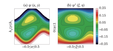
Fig.1 Streamlines mapped into (a) the physical domain $(x,y)$ and (b) the computational domain $\left( \xi, \eta \right) $ when $a=0.5,$ $% b=0.5,$ $d=1,$ $Q=1.5,$ $\phi =\pi /3, $ $M=0.9, Br=0.3$, and $\beta =0.4$. |
Consequently, for each cross-section of the geometry, the resulting dimensionless Eqs.(16) and (17) can be written in the form
$$ \qquad\quad L_{\psi ^{\ast }}\left( \psi ^{\ast },\theta ^{\ast }\right) +N_{\psi ^{\ast}}\left( \psi ^{\ast },\theta ^{\ast }\right) =0,$$
$$ \qquad\quad L_{\theta ^{\ast }}\left( \psi ^{\ast },\theta ^{\ast }\right) +N_{\theta^{\ast }}\left(\psi ^{\ast },\theta ^{\ast }\right) +BrM^{2}=0,$$
in which the linear and nonlinear parts $L_{\psi ^{\ast }}, L_{\theta ^{\ast}}, N_{\psi ^{\ast }}$, and $N_{\theta ^{\ast }}$ are given by
$$ L_{\psi ^{\ast }}\left( \psi ^{\ast },\theta ^{\ast }\right) =\frac{1}{\Delta ^{4}}\frac{\partial ^{4}\psi ^{\ast }}{\partial \eta ^{4}}-\frac{M^{2}}{\Delta ^{2}}\frac{\partial ^{2}\psi ^{\ast }}{\partial \eta ^{2}}-\frac{\beta M^{2}}{\Delta }\frac{\partial \theta ^{\ast }}{\partial \eta }, $$
$$ L_{\theta ^{\ast }}\left( \psi ^{\ast },\theta ^{\ast }\right) =\frac{1}{\Delta ^{2}}\frac{\partial ^{2}\theta ^{\ast }}{\partial \eta ^{2}}+Br\beta M^{2}\theta ^{\ast }+\frac{2BrM^{2}}{\Delta }\frac{\partial \psi ^{\ast }}{\partial \eta }, $$
$$ N_{\psi ^{\ast }}\left( \psi ^{\ast },\theta ^{\ast }\right) =-\frac{\beta M^{2}}{\Delta ^{2}}\frac{\partial \psi ^{\ast }}{\partial \eta }\frac{\partial \theta ^{\ast }}{\partial \eta }-\frac{\beta M^{2}}{\Delta ^{2}} \frac{\partial ^{2}\psi ^{\ast }}{\partial \eta ^{2}}\theta ^{\ast }, $$
$$ N_{\theta ^{\ast }}\left( \psi ^{\ast },\theta ^{\ast }\right) =\frac{Br}{\Delta ^{4}}\left( \frac{\partial ^{2}\psi ^{\ast }}{\partial \eta ^{2}} \right) ^{2}+\frac{BrM^{2}}{\Delta ^{2}}\Bigl( \frac{\partial \psi ^{\ast }}{\partial \eta }\Bigr) ^{2} +\frac{2Br\beta M^{2}}{\Delta }\frac{\partial \psi ^{\ast }}{\partial \eta }\theta ^{\ast } +\frac{Br\beta M^{2}}{\Delta ^{2}}\Bigl( \frac{\partial \psi ^{\ast }}{\partial \eta }\Bigr) ^{2}\theta^{\ast }, $$
and the modified boundary conditions take the following form
$$ \psi ^{\ast }=-F/2,\text{}\frac{\partial \psi ^{\ast }}{\partial \eta }=-\Delta ,\text{}\theta ^{\ast }=1\text{ at}\eta =0\,, \\\psi ^{\ast }=+F/2,\text{ }\frac{\partial \psi ^{\ast }}{\partial \eta }=-\Delta ,\text{ }\theta ^{\ast }=0\text{ at }\eta =1\,.$$
As mentioned above, we can express the longitudinal pressure gradient as follows
$$ \frac{{\rm d}p^{\ast }}{{\rm d}\xi }= \frac{1}{\Delta^{3}}\left. \frac{\partial^{3}\psi^{\ast }} {\partial \eta ^{3}}\right\vert _{\eta =0}-\frac{M^{2}}{\Delta }\left. \frac{\partial \psi ^{\ast }}{\partial \eta }\right\vert _{\eta=0} \\ -\beta M^{2}\theta ^{\ast }\left( \xi ,0\right) -M^{2}\,.$$
Here $p^{\ast }$ is the transformed pressure, where $p^{\ast }=p\left(f^{\ast }\left( \xi \right) \right).$
3 Solution Methodology and Validation
For solving the obtained coupled system of nonlinear partial differential equations described by Eqs. (29) and (30) and the boundary conditions (35), the generalized differential quadrature method (GDQM) is used during in this investigation as a powerful method to find out the numerical results by computing the $m^{\rm th}$-order partial derivatives with respect to $\eta $ of both $\psi ^{\ast }\left( \xi ,\eta \right) $ and $\theta ^{\ast }\left( \xi ,\eta \right) .$ Following this approach, the partial derivatives of $\psi ^{\ast }\left( \xi ,\eta \right) $ and $\theta ^{\ast }\left( \xi ,\eta \right) $ with respect to space variable $\eta $ at a given discrete point $% \eta _{i}$ can be written as follows
$$ \left.\frac{\partial^{m}\psi^{\ast}}{\partial \eta^{m}} \right\vert_{\eta=\eta_{i}}=\mathop\sum\limits^{N}_{{j=1}}d_{ij}^{(m)}\psi^{\ast}(\xi,\eta_{i})\,, $$
$$ \left.\frac{\partial ^{m}\theta^{\ast }}{\partial \eta ^{m}}\right\vert_{\eta=\eta_{i}}=\mathop\sum\limits^{N}_{{j=1}}d_{ij}^{(m)}\theta^{\ast}(\xi, \eta_{i})\,.$$
Here, $d_{ij}^{(m)}$ are the weighting coefficients for the $m^{\rm th}$-order derivative and $N$ is the total number of sampling points of the grid distribution in the transversal direction, where $i$ and $j$ are integers varying from $1$ to $N.$ According to Shu,[25] the weighting coefficients for the first-order derivative discretization with arbitrary distribution of grid points are expressed as follows
$$ d_{ij}^{(1)}=\prod\limits^{N}_{k=1,k\neq i}\left( \eta _{i}-\eta _{k}\right)/[ \left( \eta _{i}-\eta _{j}\right) \prod\limits^{N}_{k=1,k\neq j}\left( \eta _{j}-\eta _{k}\right)], $$
for $i\neq j$ and
$$ d_{ij}^{(1)}=-\sum_{{j=1,~j\neq i}}^{N}d_{ij}^{(1)},$$
for $i=j,$ where $i=1,2,3,\ldots,N.$
Similarly, the weighting coefficients of the second and higher-order derivatives can be calculated from those of the first-order derivative by the following recurrence relations
$$ d_{ij}^{(m)}=m\Bigl( d_{ii}^{(m-1)}d_{ij}^{(1)}-\frac{d_{ij}^{(m-1)}}{\eta_{i}-\eta _{j}}\Bigr),$$
for $i\neq j$ and
$$ d_{ij}^{(m)}=-\sum\limits_{{j=1,j\neq i}}^{N}d_{ij}^{(m)},$$
for $i=j,$ where $i=1,2,\ldots,N.$
In order to obtain accurate results using a few numbers of grid points $N$, it is more useful to choose the Chebyshev-Gauss-Lobatto grid points, which are greatlydenser close to the boundaries and their co-ordinates constitute the roots of the Chebyshev polynomial. These collocation points can be written in the form
$$ \eta _{i}=\frac{1}{2}\Bigl\{ 1-\cos \Bigl[ \Bigl( \frac{i-1}{N-1}\Bigr) \pi % \Bigr] \Bigr\} ,$$
where $i=1,2,\ldots,N$ and $0\leq \eta _{i}\leq 1.$ Under the above consideration, the dimensionless functions $\psi ^{\ast}\left( \xi ,\eta \right) $ and $\theta ^{\ast }\left( \xi ,\eta \right) $ are approximated in each collocation point $\eta _{i}$ by $\psi _{i}^{\ast}\left( \xi \right) $ and $\theta _{i}^{\ast }\left( \xi \right) ,$ respectively. Hence, after discretizing the transformed problem with some rearrangements, Eqs. (29) and (30) together with the boundary conditions (35) are simplified as
$$ \left( S\right):\cases\psi _{i}^{\ast }\left( \xi \right) + {F}/{2}=0\,, \quad\mathop\sum\limits^{N}_{{j=1}}d_{ij}^{(1)}\psi _{j}^{\ast }\left( \xi\right) +\Delta =0\,,L_{\psi _{i}^{\ast }}\left( \psi _{i}^{\ast }\left( \xi \right),\theta_{i}^{\ast }\left( \xi \right) \right) +N_{\psi _{i}^{\ast }}\left( \psi_{i}^{\ast }\left( \xi \right),\theta _{i}^{\ast }\left( \xi \right)\right)=0\,,\hfill\cr\quad 3\leq i\leq N-2\,,\hfill\cr\mathop\sum\limits^{N}_{{j=1}}d_{Nj}^{(1)}\psi _{j}^{\ast }\left( \xi\right) +\Delta =0\,, \quad\psi _{N}^{\ast }\left( \xi \right) - {F}/{2}=0\,,\hfill\cr\theta _{i}^{\ast }\left( \xi \right) -1=0\,,L_{\theta _{i}^{\ast }}\left( \psi _{i}^{\ast }\left( \xi \right),\theta_{i}^{\ast }\left( \xi \right) \right) +N_{\theta _{i}^{\ast }}\left( \psi_{i}^{\ast }\left( \xi \right),\theta _{i}^{\ast }\left( \xi \right)\right)\hfill\cr +\,BrM^{2}=0,\quad 2\leq i\leq N-1,\hfill\cr\theta _{N}^{\ast }\left( \xi \right) =0\,,}$$
where
$$ L_{\psi _{i}^{\ast }}\left( \psi _{i}^{\ast },\theta _{i}^{\ast }\right) =\frac{1}{\Delta ^{4}}\mathop\sum\limits^{N}_{{j=1}}d_{ij}^{(4)}\psi _{j}^{\ast }-\frac{M^{2}}{\Delta ^{2}}\mathop\sum\limits^{N}_{{j=1}} d_{ij}^{(2)}\psi _{j}^{\ast } -\frac{\beta M^{2}}{\Delta } \mathop\sum\limits^{N}_{{j=1}}d_{ij}^{(1)}\theta _{j}^{\ast },$$
$$ L_{\theta _{i}^{\ast }}\left( \psi _{i}^{\ast },\theta _{i}^{\ast }\right) = \frac{1}{\Delta ^{2}}\mathop\sum\limits^{N}_{{j=1} }d_{ij}^{(2)}\theta_{j}^{\ast }+Br\beta M^{2}\theta _{i}^{\ast }+\frac{2BrM^{2}}{\Delta } \mathop\sum\limits^{N}_{{j=1}}d_{ij}^{(1)}\psi _{j}^{\ast },$$
$$ N_{\psi _{i}^{\ast }}\left( \psi _{i}^{\ast },\theta _{i}^{\ast }\right) =-\frac{\beta M^{2}}{\Delta ^{2}}\Bigl( \mathop\sum\limits^{N}_{{j=1}}%d_{ij}^{(1)}\psi _{j}^{\ast }\Bigr) \Bigl( \mathop\sum\limits^{N}_{{j=1}%}d_{ij}^{(1)}\theta _{j}^{\ast }\Bigr)-\frac{\beta M^{2}}{\Delta ^{2}} \Bigl( \mathop\sum\limits^{N}_{{j=1}}d_{ij}^{(2)}\psi _{j}^{\ast}\Bigr) \theta _{i}^{\ast }\,,$$
$$ N_{\theta _{i}^{\ast }}\left( \psi _{i}^{\ast },\theta _{i}^{\ast }\right)=\frac{Br}{\Delta ^{4}}\Bigl( \mathop\sum\limits^{N}_{{j=1}} d_{ij}^{(2)}\psi _{j}^{\ast }\Bigr) ^{2} \! \!+\frac{BrM^{2}}{\Delta ^{2}}\Bigl(\mathop\sum\limits^{N}_{{j=1}}d_{ij}^{(1)}\psi _{j}^{\ast }\Bigr) ^{2}\!+\!\frac{2Br\beta M^{2}}{\Delta }\Bigl( \mathop\sum\limits^{N}_{{j=1}} d_{ij}^{(1)}\psi _{j}^{\ast }\Bigr) \theta _{i}^{\ast }+\frac{Br\beta M^{2}}{\Delta ^{2}}\Bigl( \mathop\sum\limits^{N}_{{j=1}} d_{ij}^{(1)}\psi _{j}^{\ast }\Bigr) ^{2}\theta _{i}^{\ast }.$$
$$ \frac{{\rm d}p^{\ast }}{{\rm d}\xi }=\frac{1}{\Delta ^{3}}\mathop\sum\limits^{N}_{{j=1}}d_{1j}^{(3)}\psi _{j}^{\ast }-\frac{M^{2}}{\Delta }\mathop\sum\limits^{N}_{{j=1}{ }}d_{1j}^{(1)} \psi _{j}^{\ast }-\beta M^{2}\theta_{1}^{\ast }-\frac{\beta M^{2}}{\Delta }\Bigl( \mathop\sum\limits^{N}_{{j=1}}d_{1j}^{(1)}\psi _{j}^{\ast }\Bigr) \theta _{1}^{\ast }-M^{2}\,.$$
As shown above, the numerical procedure used in this investigation leads to a nonlinear system $\left( S\right) $ constituted by $2N$ algebraic equations, which can then be solved using an algorithm based on the Newton-Raphson technique.
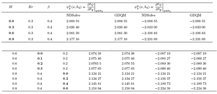
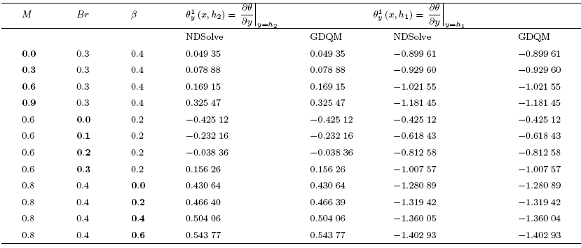
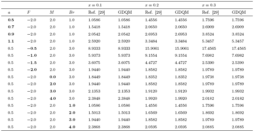
To validate our numerical computations and test the efficiency of the proposed method, several tabular and graphical comparisons are carried out, in order to obtain a reliable physical prediction. In Tables 1 and 2, we present a comparison of the engineering quantities $\psi _{y}^{\left( 2\right) }\left( x,h_{2}\right) ,$ $\psi _{y}^{\left( 2\right) }\left( x,h_{1}\right) ,$ $\theta _{y}^{\left( 1\right) }\left( x,h_{2}\right) $, and $\theta _{y}^{\left( 1\right) }\left( x,h_{1}\right) $ obtained by the help of the Mathematica's NDSolve function and the generalized differential quadrature method (GDQM), for various parametric values $M,$ $Br$ and $% \beta ,$ when $a=0.5,$ $b=0.5,$ $d=1,$ $Q=1.5,$ $x=0.1$, and $\phi =\pi /3.$ As expected, it is found an excellent agreement in term of the absolute accuracy of the order of $10^{-6}$ between both methods, when we choose $N=50 $ as the number of collocation points. Hence, the tabular results confirm the validity of our numerical code and the effectiveness of the generalized differential quadrature method (GDQM). More, comparison of present results with the existing study is presented in Table 3. The obtained results are found to be in an excellent agreement.
Tab. 1 Comparison between our numerical results and those given by software for $\psi _{y}^{2}\left( x,h_{2}\right) $ and $\psi _{y}^{2}\left( x,h_{1}\right) $ in the case where $% a=0.5,b=0.5,d=1,Q=1.5,x=0.1$ and $\phi =\pi /3.$ |
 |
Tab. 2 Comparison between our numerical results and those given by software for $\theta _{y}^{1}\left( x,h_{2}\right) $ and $% \theta _{y}^{1}\left( x,h_{1}\right) $ in the case where $% a=0.5,b=0.5,d=1,Q=1.5,x=0.1$ and $\phi =\pi /3.$ |
 |
Tab. 3 Comparison between our numerical results and the results of Srinivas and Kothandapani[29] for the ideal heat transfer coefficient $% Z=h_{1}^{(1)}\theta _{y}^{(1)}\left( x,h_{1}\right) $ in the case where $% \beta =0,b=0.6,d=1.5$ and $\phi =\pi /4.$ |
 |
4 Results and Discussions
This section is devoted to analyze and discuss the behavior of velocity profile $u\left( x,y\right),$ temperature profile $\theta \left(x,y\right)$, pressure gradient ${\rm d}p/{\rm d}x$ and streamlines on varying the dominating physical parameters appearing in the flow problem like Hartmann number $M,$ electrical conductivity parameter $\beta,$ and Brinkman number $Br.$ In Fig.2 velocity profiles $u$ are plotted for various values of Hartmann number $M$. It is obvious to note that velocity profile $u$ is decreasing centrally but increasing slightly near the walls of channel when Hartmann number $M$ is steadily increased. This happens because, the magnetic field interacts with the electrically conducting fluid and generate a Lorentz force which is opposite in the direction of fluid flow and therefore, the fluid velocity decreases. Since the electrical conductivity parameter $\beta $ appears due to the Lorentz force in momentum equation, it might affect in the same way as does the Hartmann number $M$. Its effect on velocity profile $u$ is exhibited in Fig.3, wherein velocity profile $u$ is seen to be weakened on strengthening the intensity of electrical conductivity.
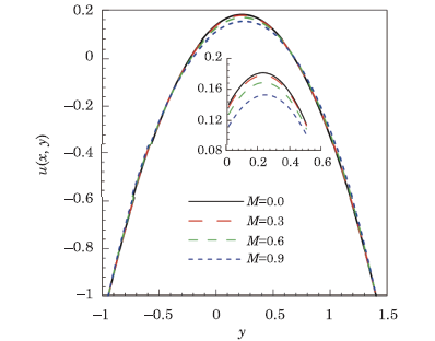
Fig.2 Velocity profile $u\left( x,y\right) $ for different values of Hartmann number $M$, when $a=0.5,$ $b=0.5,$ $d=1,$ $Q=1.5,$ $x=0.1,$ $ \phi =\pi /3,$ $Br=0.3$, and $\beta =0.4.$ |
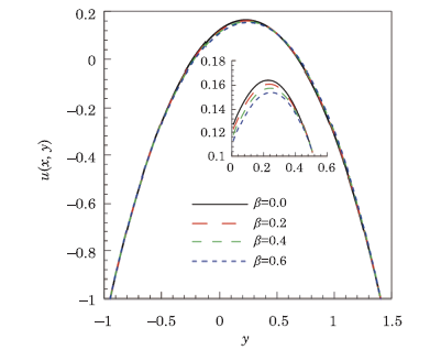
Fig.3 Velocity profile $u\left( x,y\right) $ for different values of electrical conductivity parameter $\beta $, when $a=0.5,$ $b=0.5,$ $d=1,$ $Q=1.5,$ $x=0.1,$ $\phi =\pi /3,$ $Br=0.3$, and $M=0.8.$ |

Fig.4 Temperature profile $\theta \left( x,y\right) $ for different values of Hartmann number $M$, when $a=0.5,$ $b=0.5,$ $d=1,$ $Q=1.5,$ $x=0.1,$ $\phi =\pi /3,$ $Br=0.3$, and $\beta =0.4.$ |
Figure 4 presents the analysis of temperature profile $\theta $ against the increasing values of Hartmann number $M$. Physically, increasing values of decelerate the fluid flow consequently the friction between the fluid layers increases and generates frictional heating, which enhances the temperature. It is noticed that down the stream temperature is decreasing because of increasing values of Hartmann number $M$. Similar effects on temperature profile $\theta $ are observed in case of increasing electrical conductivity parameter $\beta $, shown in Fig.5. Brinkman number $Br$ appears in heat equation due the dissipation term. In the flow process kinetic energy is converted into heat energy due to viscous dissipation and increasing Brinkman number $Br$ is same as to increase the heat energy. Thus Fig.6 follows the trend of increasing temperature on increasing the values of Brinkman number $Br$.
Figure 7 is drawn to study the effects of Hartmann number $M$ on pressure gradient. Here pressure gradient may be classified as the adverse pressure gradient and favorable pressure gradient on being positive and negative respectively. From this figure we note that pressure gradient is increasing in the domain $[-0.4,0]$ and $[0.4,1.0]$ while decreasing in $[-1.0,-0.4]$ and $[0,0.4].$ Overall pressure gradient is decreasing in magnitude on the increase in Hartmann number $M$.
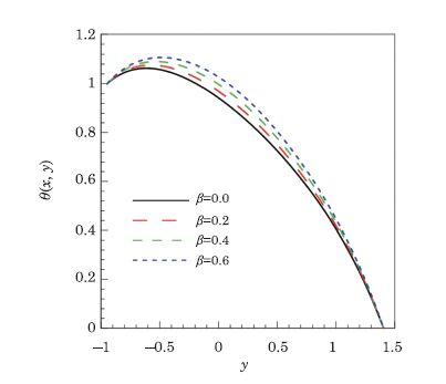
Fig.5 Temperature profile $\theta \left( x,y\right) $ for different values of electrical conductivity parameter $\beta $, when $a=0.5,$ $b=0.5,$ $d=1,$ $Q=1.5,$ $x=0.1,$ $\phi =\pi /3,$ $Br=0.3$, and $M=0.8.$ |
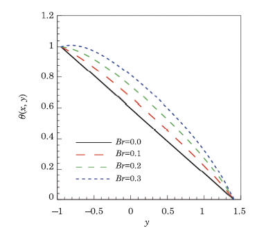
Fig.6 Temperature profile $\theta \left( x,y\right) $ for different values of Brinkman number $Br$, when $a=0.5,$ $b=0.5,$ $d=1,$ $Q=1.5,$ $x=0.1,$ $\phi =\pi /3,$ $\beta =0.3$, and $M=0.6.$ |
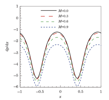
Fig.7 Variation of pressure gradient ${\rm d}p/{\rm d}x$ for different values of Hartmann number $M$, when $a=0.5,$ $b=0.5,$ $d=1,$ $Q=1.5,$ $x=0.1,$ $ \phi =\pi /3,$ $Br=0.3$, and $\beta =0.4.$ |
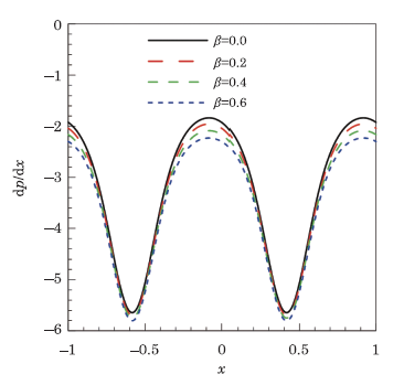
Fig.8 Variation of pressure gradient ${\rm d}p/{\rm d}x$ for different values of electrical conductivity parameter $\beta $, when $a=0.5,$ $b=0.5,$ $d=1,$ $Q=1.5,$ $x=0.1,$ $\phi =\pi /3,$ $Br=0.4$, and $\beta =0.8.$ |
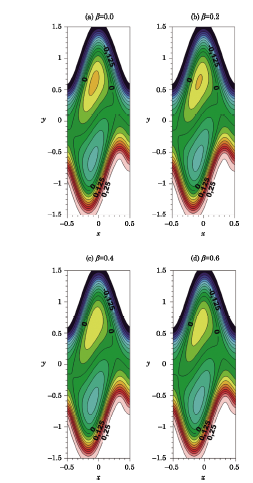
Figure 8 shows the behavior of pressure gradient when electrical conductivity parameter $\beta $ is given boost. It is noticeable that strengthening the intensity of electrical conductivity, the same effects of decreasing pressure gradient are observed.Since the electrical conductivity parameter $\beta $ contributes in Lorentz force and Joule heating so its effects might be the same as to that of magnetic number and Joule heating parameter.The phenomenon of trapping in peristalsis is the split of streamlines and formation of a bolus when the fluid is moving in wave frame. Figures 9 and 10 are exhibited to observe the effects of Hartmann number $M$ and electrical conductivity parameter $\beta $ respectively. In both figures volume of trapped bolus is observed to be decreasing subsequently on increasing the Hartmann number $M$ and electrical conductivity parameter $\beta $. Initially bolus is seen to be formed centrally in the absence of magnetic field and electrical conductivity. Gradually strengthening both the factors,trapped bolus is seen to shift to upward boundary of the channel and eventually disappears on increasing Hartmann number $M$ and electrical conductivity parameter $\beta$.
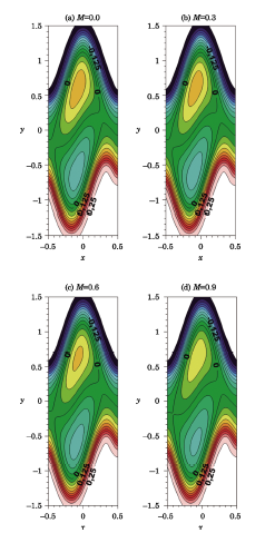
Fig.9 Streamlines for different values of Hartmann number $M$,when $a=0.5,$ $b=0.5,$ $d=1,$ $Q=1.5,$ $x=0.1,$ $\phi =\pi /3,$ $Br=0.3$, and $\beta =0.4.$ |
Fig.10 Streamlines for different values of electrical conductivity parameter $\beta $, when $a=0.5,$ $b=0.5,$ $d=1,$ $Q=1.5,$ $x=0.1,$ $\phi =\pi /3,$ $Br=0.4$, and $M=0.8.$ |