


1 Introduction
In a hyper-connected world,[1] the functions of many complex systems, like power grid or transportation networks, depend on their structures and scales. The breaking of structural connectivity may result in functional failure.[2-4] For example, to confine the epidemic spreading, an effective way is vaccinating the people who can dismantle the infection network as far as possible.[5-7] These scenarios equal to the network dismantling problem: For a graph $\mathcal{G}$ with $N$ nodes, how to find the minimum separate set of nodes whose removal will break the graph into numerous connected components with sub-extensive size, which means the size of the largest connected component cannot be larger than the threshold $0.01N$.[8-9] The studies on this problem are of both theoretical importance[10-12] and practical significant.[13-15]
It has been proved that the dismantling problem belongs to the NP-hard class, which means, in the general case, we cannot find the minimum separate set by a polynomial algorithm. However, many heuristic strategies have been developed based on various graph properties. For example, we can use many centrality measures to quantify the importance of nodes,[16-19] and repeatedly deleting the most important one, such as the node with the highest degree[14] or with the highest betweenness.[20] Previous study showed that comparing with the deletion of the highest degree node in the original graph, a better choice is deleting the highest degree node in the 2-core of the graph —— the largest sub-graph where the nodes' residual degree are no less than 2 after repeatedly removing all leaf nodes.[21] Another development of the algorithm in the same category is to quantify the collective influence of nodes through optimum percolation on networks.[22] The removal of nodes with the highest collective influence will dismantle the network fastly. In addition, the study of the dismantling problem on weighted network showed that some of the state-of-the-art algorithms are of low efficiency, even worse than random attacking method.[9,23]
Recently, Mugisha and Zhou pointed out that the network dismantling problem relates to the spanning forest problem, which is also referred as the feedback vertex set (FVS) problem.[24] Therefore, a near-optimum solution of network dismantling problem can be found through belief-propagation guided decimation (BPD) algorithm (see Sec. 2 for more details). Along similar lines, Braunstein et al. also developed a Min-Sum algorithm to decycle and dismantle networks.[8] The FVS class algorithms have proved itself in finding the near minimum separate set, but there is still improvement space during the dismantling process. Because these algorithms remove nodes in the purpose of decycling instead of network dismantling, which results in the size of the largest connected component decreasing slowly before its abrupt drop at the threshold value.
Different from only asking the minimum separate set of a dismantling problem, we also concern about the order of how they are removed from the graph, which will decide the general efficiency of a dismantling algorithm. If we attack a graph according to a dismantling sequence with high general efficiency, the largest connected component in the remaining graph will break as quickly as possible. In this paper, we propose a practicable framework to improve the general efficiency of a dismantling algorithm via the node explosive percolation (NEP) algorithm.[25-27] Take the BPD algorithm as an example, we introduce an NEP-BPD algorithm, called NBA for short, which will reorder the first a few nodes of a dismantling sequence given by the BPD algorithm. Experimental results on both modeled and real networks indicate that the new method greatly improves the general efficiency of the early part of the original dismantling sequence, and does not lead to any degeneration at the later part.
This paper is organized as follows: In Sec. 2, we firstly introduce two criteria to evaluate the dismantling efficiency and the general efficiency of a dismantling algorithm. Then we review the BPD and the NEP algorithms in detail. Finally, we show how to link two methods together to form the NBA algorithm. In Sec. 3, we measure the ability of the NBA in improving the general efficiency numerically on modeled networks, including the Erdös-Rényi (ER) graphs, random-regular (RR) graphs, and scale-free (SF) graphs. In order to reduce the computational complexity of NBA, we further investigate the relationship between the number of reordered node and the general efficiency of the NBA. The result of this study helps us implement the fast NBA —— a compromise algorithm under limited computing resources. Finally, we apply the fast NBA in all random graph ensembles and some real networks. In the last section, we conclude the new method, summarize the main results, and discuss possible extensions of the method.
2 Method
For a graph $\mathcal{G}$ with $N$ nodes, after removing $\rho N$ $(0\le \rho \le 1)$ nodes and their adjacent edges from the graph, the relative size of the largest connected component in the remaining graph is denoted as $g(\rho)$. There are two aspects to evaluate the efficiency of a dismantling algorithm: One aspect considers the size of the minimum separate set. A wildly applied criterion is the dismantling efficiency $\rho_c$, which is defined as the smallest value of $\rho$ where $g(\rho)\leq 0.01$.[8,22,24,27] The other is the removing order of the removed nodes. A good dismantling algorithm will give a dismantling sequence in which every node removal leads to the maximum damage in the remaining graph. In the present paper, we introduce the average size fraction of the largest connected components $R$ to evaluate the general efficiency of a dismantling algorithm:[25-26]
$R = \int_0^1 g(\rho) d \rho.$
We can see that, an algorithm with higher general efficiency algorithm gives a smaller $R$.
In order to highlight the advancement of the NBA compared with the BPD, we define the relative improvement of the $R$, which reads
$r=\frac{R^{\rm{BPD}}-R^{\rm{NBA}}}{R^{\rm{BPD}}}\times 100 \%,$
where $R^{\rm{BPD}}$ and $R^{\rm{NBA}}$ are the value of $R$ given by the BPD and NBA respectively. In the following subsections, we will firstly review the BPD and NEP algorithms, and then explain how to implement the NBA in detail.
2.1 The BPD Algorithm for Dismantling Problem
Dismantling algorithms based on the FVS attacking strategy, such the BPD algorithm and the Min-Sum algorithm, are composed of three main stages: Firstly, finding the minimum FVS of graph $\mathcal{G}$ by the minimum FVS algorithm. After all nodes in the FVS are removed from the graph, the remaining graph becomes acyclic. Secondly, continue breaking the remaining forest in the most efficient way. In the above two steps, the algorithm builds a dismantling sequence $(x_i)$ based on the order of the node removal. The first $N\rho_c$ nodes in the sequence form the separate set. In the last step, in order to minimize the separate set, we can move some nodes in the separate set which will not lead to the increase of the size of the largest connected component to the end of the sequence.
In the first stage, the BPD algorithm translates the FVS problem with global constraint to a spin-glass model containing only local constraint.[28-29] For each node $i$, it defines a state $A_i\in\{0, i, j\in\partial i\}$, which means the node $i$ is not in the FVS, the root of a tree or the child of its neighboring node $j$ respectively. Then the long-range constraint of no loop in the graph can be replaced by a series of local constraints on edges:
$C_{(i,j)}(A_i,A_j) \equiv \delta^0_{A_i}\delta^0_{A_j} +\delta^0_{A_i}(1-\delta^0_{A_j}-\delta^i_{A_j}) +\delta^0_{A_j}(1-\delta^0_{A_i} \\ -\delta^j_{A_i})+\delta^j_{A_i} (1-\delta^0_{A_j}-\delta^i_{A_j}) + \delta^i_{A_j}(1-\delta^0_{A_i} \\ -\delta^j_{A_i}), $
where $\delta_x^y$ is the Kronecker symbol such that $\delta_x^y=1$ only when $x=y$, otherwise $\delta_x^y=0$.
Therefore, only when $A_i$ and $A_j$ satisfy the constraint on edge $(i,j)$, $C_{(i,j)}(A_i,A_j)=1$. If a microscopic configuration $\underline{A}\equiv (A_1,A_2,\ldots,A_N)$ satisfies all constraints in $\mathcal{G}$, we refer it as the legitimate configuration. If we remove all nodes with $A_i = 0$ in a legitimate configuration $\underline{A}$ from $\mathcal{G}$, the remaining graph contains only trees and a few cycle-trees, which is a kind of subgraph with only one loop. Therefore, the set of nodes with $A_i = 0$ in a legitimate configuration can be regarded as an FVS approximately. The energy of $\underline{A}$, corresponding to the size of the FVS, is defined as the number of nodes with $A_i = 0$:
$E(\underline{A})=\sum_i \delta^0_{A_i}.$
If the spin-glass system follows the Boltzmann distribution, the probability of observing a legitimate configuration $\underline{A}$ is
$p(\underline{A})=\frac{ e^{-\beta E(\underline{A})}}{Z(\beta)},$
where $\beta$ is the inverse temperature and $Z(\beta)$ is the partition function
$Z(\beta)=\sum_{\underline{A}} \prod_{(i,j)\in\mathcal{G}} C_{(i,j)}(A_i,A_j) e^{-\beta E(\underline{A})}. $
In order to find a ground state of this spin-glass model, the BPD algorithm follows the standard steps of the cavity method by defining a pair of messages (probability distribution) on each edge $(i,j)\in\mathcal{G}$: $q^A_{i\rightarrow j}$ and $q^A_{j\rightarrow i}$, where $q^A_{i\rightarrow j}$ is the marginal probability of node $i$ taking the state $A$ in the absence of node $j$. Considered the constraint Eq. (3), all messages in the graph $\mathcal{G}$ should fulfill the following belief-propagation equations:
$q^0_{i\rightarrow j}= \frac{ e^{-\beta}}{z_{i\rightarrow j}},$
$q^i_{i\rightarrow j} = \frac{1}{z_{i\rightarrow j}} \prod_{k \in \partial i\backslash j}( q^0_{k\rightarrow i}+q^k_{k \rightarrow i}),$
$q^l_{i\rightarrow j} = \frac{1-q^0_{l\rightarrow i}}{z_{i\rightarrow j}} \prod_{k \in \partial i\backslash j,l} ( q^0_{k\rightarrow i}+q^k_{k \rightarrow i}\bigr) \,, \quad (l\in \partial i \backslash j) $
where $\partial i\setminus j$ means the vertex set obtained by deleting vertex $j$ from $\partial i$ and the normalization factor $z_{i\to j}$ is
$z_{i\rightarrow j}\equiv e^{-\beta}+ \Bigl(1+\sum_{k \in \partial i\backslash j} \frac{1-q^0_{k\rightarrow i}}{q^0_{k\rightarrow i}+q^k_{k \rightarrow i}} \Bigr) \\ \times\prod_{l \in \partial i\backslash j} ( q^0_{l\rightarrow i}+q^l_{l \rightarrow i}).$
Therefore, the marginal probability of node $i$ taking the state 0 in $\mathcal{G}$ is,
$q_i^0 = [1+ e^{\beta} \Bigl( 1+\sum_{k \in \partial i} \frac{1-q^0_{k\rightarrow i}}{q^0_{k\rightarrow i}+q^k_{k \rightarrow i}} \Bigr) \\ \times\prod_{j \in \partial i}(q^0_{j\rightarrow i} +q^j_{j \rightarrow i})\Bigr]^{-1}.$
The BPD algorithm can figure out which node should take the state $A=0$ by repeating the following two steps until there are only trees or cycle-trees left in the remaining graph: (i) Iterate Eqs. (7)-(9) with large $\beta$ on graph $\mathcal{G}$ to propagate these messages as far as possible and then compute $q_i^0$ for each node by Eq. (11). (ii) Delete a small fraction of nodes with the largest $q_i^0$ from the graph. Then, continue breaking cycle-trees by attacking any one node on the cycle. In the following discussion, we use $\mathcal{T}_\alpha$ to denote the tree $\alpha$ in the remaining forest $\mathcal{F}$.
In the second stage, the $\mathcal{F}$ will be broken as quickly as possible. To achieve this purpose, it defines another pair of messages on each edge $(i,j)\in\mathcal{F}$: $n_{i\rightarrow j}$ and $n_{j\rightarrow i}$. $n_{i\rightarrow j}$ saves the size of the remaining tree containing node $i$ after cutting edge $(i,j)$. It is obvious that $n_{i\rightarrow j}=1$ if $i$ is a leaf node. The iteration equations of these messages read
$n_{i\rightarrow j}=1+\sum_{k\in \partial i\setminus j} n_{k \rightarrow i}.$
These equations can be solved easily by starting from all leaf nodes and then propagating to the whole tree gradually.
If a node $i\in\mathcal{T}_\alpha$ is attacked, $\mathcal{T}_\alpha$ will break into a few smaller trees with the size $\{n_{j\rightarrow i}\}_{j\in \partial i}$, in which the size of the largest one is denoted by
$n_i=\max\limits_{j \in \partial i} n_{j \rightarrow i}.$
Therefore, the most efficient way of breaking $\mathcal{T}_\alpha$ is to attack the node with the smallest $n_i$. Moreover, in order to quickly decrease the size of the largest connected component, we should firstly dismantle the largest tree in $\mathcal{F}$. By repeatedly removing the node with the minimum $n_i$ in the largest tree, a forest with giant trees will break into many tiny trees with the size no larger than the threshold value $0.01N$. The remaining forest can be broken further until all nodes are removed.
If we dismantle the graph according to the sequence $(x_i)$, after $N\rho_c$ nodes are removed, there will be a mass of connected components whose size are much smaller than the threshold value. In order to find out the minimum separate set, we can recover some removed nodes back to the remaining graph in the last step, which will not lead to the increase of the size of the largest connected component. At the same time, the recovered nodes are moved to the end of the dismantling sequence.
The fact that the BPD algorithm performs good in giving a small $\rho_c$ indicates its high dismantling efficiency. However, as discussed in Sec. 1, this kind of algorithms, including BPD algorithm, Min-Sum algorithm, equal graph partitioning algorithm,[30] {etc}., suffer from a low general efficiency problem related to the fact that the value of $g(\rho)$ decreases slowly before its abrupt drop at $\rho_c$. Therefore, the general efficiency of these algorithms can be further improved by reordering their dismantling sequences.
2.2 The NEP Algorithm for Dismantling Problem
Different from most traditional dismantling algorithms, the NEP algorithm solves this problem using a backward thinking. It starts from a dismantled graph (i.e., a residual graph after the removing of a specific part of nodes) and then recovers the node with its attached edges. During the recovering process, some small connected components merge to a bigger one. The NEP restores the node who can largely prevent increase of the largest connected component. Finally, the NEP gives a dismantling sequence in the reverse order of the restoring process, which reduces the size of the largest connected component as quickly as possible.
In the NEP algorithm, a score $\sigma_i$ measuring the ability of node $i$ merging neighbouring connected components is defined. The node with the minimum $\sigma_i$ should be recovered to the dismantled graph with priority. If more than one node have the minimum score, we randomly select one in them. After all removed nodes are recovered, we assemble the original graph back and generate a complete dismantling sequence.
The performance of the NEP algorithm depends on the definition of $\sigma_i$, which considers all neighbouring connected components of node $i$. For example, in the simplest way,[25] $\sigma_i$ can be defined as the size of the connected component built by restoring node $i$ to the remaining graph. We denote the above recovering targeting algorithm as the NEP with definition 1 (${\rm NEP}^1$), namely
$\sigma_i=\sum_j {\cal{M}}_{i,j} + 1,$
where ${\cal{M}}_{i,j}$ is the size of the $j$-th largest neighbouring connected component of node $i$.
Although the ${\rm NEP}^1$ prevents the increase of the size of the largest connected component in the present, it may lead to an unexpected great increase when two large connected components join together in the future. In order to overcome the drawback in ${\rm NEP}^1$, we also adopt the second score definition (${\rm NEP}^2$),[27]
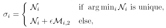
where $\mathcal{N}_i$ is the number of neighbouring connected components of node $i$, ${\cal{M}}_{i,2}$ is the size of the second largest neighbouring connected component of node $i$, $\epsilon$ is a very small positive number ($\epsilon \ll 1/N$). Therefore, ${\rm NEP}^2$ prefers to recover the node with fewer neighbouring connected components. If more than one node have the same minimum $\mathcal{N}_i$, the node with the smallest ${\cal{M}}_{i,2}$ will be selected.
2.3 The NEP-BPD Algorithm
A useful property in dismantling problem is that after a part of nodes are removed from a graph, the structure of the remaining graph is merely decided by the set of the removed nodes while independent of the order of the removal process. Moreover, the NEP algorithm can reorder the first $T$ elements of a dismantling sequence, which might improve the general efficiency of the first $T$ steps without any negative impact on the rest part. Therefore, we can take this advantage of the NEP algorithm to optimize a dismantling sequence generated by the BPD algorithm according to the following steps. Firstly, we use BPD algorithm to find a dismantling sequence $(x_i)_{i=1}^N$. Then, we split $(x_i)_{i=1}^N$ into two parts at $T$: the early part $(x_i)_{i=1}^T$ and the later part $(x_i)_{i=T+1}^N$. We remove the nodes in the early part from $\mathcal{G}$ and keep other nodes unchanged in the remaining graph. Next, we use ${\rm NEP}^1$ or ${\rm NEP}^2$ on the remaining graph to recover and reorder the nodes in the early part. At last, we obtain a complete dismantling sequence with higher general efficiency by reconnecting the reordered early part and the later part together. We use ${\rm NBA}^1$ and ${\rm NBA}^2$ to denote the NBA with ${\rm NEP}^1$ and ${\rm NEP}^2$, respectively.
The last question in the NBA is how to find out the best point $T$ where we split the original sequence $(x_i)_{i=1}^N$. According to the criteria $\rho_c$ and $R$, which are used to evaluate the performance of a dismantling algorithm, we should choose the split point $T$ where one or both criteria can be optimized. However, in most cases, $\rho_c$ and $R$ cannot be minimized simultaneously. Therefore in this paper we mainly focus our attention on the general efficiency and minimizing $R$ with due consideration of the $\rho_c$. Sometimes, merely optimizing $R$ might lead to a certain degeneration of $\rho_c$. When dismantling efficiency is more important in some problems, we can also choose $T$ with the minimum $R$ on the condition of $\rho^{\rm{NBA}}_c\leq\rho^{\rm{BPD}}_c$.
3 Results
In this section, we evaluate the performance of the NBA on three different random graph ensembles: ER graph, RR graph, and SF graph with power-law exponent $\gamma=3.0$. In the present paper, we generate the SF networks by a static method explained in Ref. [31]. Without being specific, the results in the following discussion are obtained by averaging over 16 different graph instances with $N=2^{16}$. Comparing with the results of the original BPD algorithm, we find that the general efficiency can be improved conspicuously by NBA.
Figure 1 presents the relative size of the largest connected component $g$ as a function of the fraction of the removed nodes $\rho$, given by various algorithms on an ER graph instance with average degree $\langle k\rangle=4.0$ and another RR graph instance with degree $k=4$. We can observe that the BPD algorithm gives a very small $\rho_c^{\rm{BPD}}=0.2162$ in the ER graph and $\rho_c^{\rm{BPD}}=0.3346$ in the RR graph. For comparison, the ${\rm{NEP^1}}$ and ${\rm{NEP^2}}$ give $\rho_c^{\rm{NEP^1}}=0.2468$, $\rho_c^{\rm{NEP^2}}=0.2625$ in the ER graph and $\rho_c^{\rm{NEP^1}}=0.3435$, $\rho_c^{\rm{NEP^2}}=0.3538$ in the RR graph, respectively. Although the NEP algorithms are not good at giving a small dismantling set, they are superior to the BPD algorithm in the region $\rho<\rho_c^{\rm{BPD}}$. The ${\rm NEP^2}$ has a better general efficiency than the BPD. The BPD algorithm gives $R^{\rm BPD}=0.1852$ and $R^{\rm BPD}=0.2777$ for the ER and RR graph, respectively, compared with those of the ${\rm NEP^2}$: $R^{\rm{NEP^2}}=0.1773$ and $R^{\rm{NEP^2}}=0.2397$. However the general efficiency $R$ of the NBA is the smallest among all tested algorithms, which reaches $R^{\rm{NBA^1}}=0.1708$, $R^{\rm{NBA^2}}=0.1611$ on the ER graph and $R^{\rm{NEP^1}}=0.2570$ and $R^{\rm{NBA^2}}=0.2351$ on the RR graph. Note that the improvement of the general efficiency in NBA might be accompanied with the degeneration of $\rho_c$. However, in our experiments we only observe a little increase of $\rho_c$ ($0.03%$) in the RR graph for the ${\rm NBA^2}$ compared with $\rho_c^{\rm{BPD}}$. Therefore, the negative impacts of improving general efficiency in NBA is negligible.
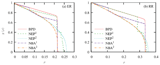
Fig. 1 (Color online) The relative size of the largest connected component $g$ in an ER graph with average degree $\langle k\rangle=4.0$ (a) and an RR graph with $k=4$ (b) with the fraction of removed node $\rho$. In these figures, we present the result of BPD algorithm (solid line), the ${\rm{NEP^1}}$ and ${\rm{NEP^2}}$ algorithm (dashed line and dotted line), and the ${\rm{NBA^1}}$ and ${\rm{NBA^2}}$ (dashed-dotted line and dashed-dotted-dotted line). |
In order to highlight the advantage of the NBA, we investigate the value of $R$ and $r$ on ER, RR, and SF graph ensembles with various degree distributions systematically, and present the results in Fig. 2. On all graph ensembles, the BPD gives the worst general efficiency in all tested algorithms and the NBA raises general efficiency in different degree. Although the relative improvement $r$ decreases with growing connectivity in most cases except when we apply the ${\rm{NBA^2}}$ sparse SF graphs ($\langle k\rangle<7$), there still exist conspicuous improvement in the NBA. We also find that ${\rm{NBA^2}}$ is more powerful than ${\rm{NBA^1}}$ in improving the general efficiency except for the SF graph when $\langle k\rangle<3$.
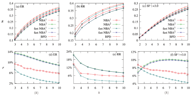
Fig. 2 (Color online) The general efficiency $R$ for the ER graph (a), RR graph (b) and for SF graph with power-law exponent $\gamma=3.0$ (c) as the function of average degree $\langle k \rangle$. We present the results of BPD algorithm, ${\rm{NBA^1}}$, ${\rm{NBA^2}}$, the fast ${\rm{NBA^1}}$ and fast ${\rm{NBA^2}}$. (d), (e), and (f) are the relative improvement $r$ of these algorithms. |
Based on the description of the NBA in the above section, it seems that we should repeat the NEP algorithm $N$ times to find the best $T\in[1,N]$ where $R$ reaches its minimum. In that case, the NBA will be at least $N$ times slower than the NEP. Considered the cost of the computation time, the price of the improvement earned by NBA seems to be too expensive. In order to avoid the expanding of the computation cost, it is necessary to reduce the searching space of $T$. For this purpose, we study the dependence of $R^{\rm NBA}$ on the number of reordered nodes and present the results in Fig. 3. It shows that the value of $R$ of ${\rm{NBA}^2}$ decreases with growing $T$ monotonically when $T<N\rho_c^{\rm{BPD}}$ and keeps stable when $T\geq N\rho_c^{\rm{BPD}}$. For ${\rm{NBA}^1}$, except for the RR graph with $k=3$, $R$ decreases with $T$ first and then increase quickly to a stable value. Moreover, the minimum $R$ appears at $T<N\rho_c^{\rm{BPD}}$. Therefore, we do not have to compute and compare the value of $R$ through the entire searching space $T\in[1,N]$, but only need to focus our attention in a very narrow region around $N\rho_c^{\rm{BPD}}$. For example, in order to save computation time as much as possible, we can set $T=N\rho_c^{\rm{BPD}}$ directly in the NBA, which is denoted as the fast NBA here. We also use the fast ${\rm{NBA}^1}$ and fast ${\rm{NBA}^2}$ to denote two fast NBA algorithms with score definition 1 and 2. In other words, the fast NBA reorders all nodes in the separate set given by the BPD algorithm. Therefore, it inherits the high dismantling efficiency in the BPD algorithm because the separate set is completely given by the BPD.
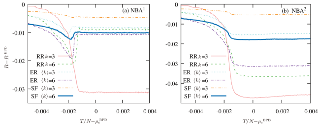
Fig. 3 (Color online) The comparison of the general efficiency $R$ between the BPD algorithm and ${\rm{NBA^1}}$ (a) and ${\rm{NBA^2}}$ (b) in the function of the number of reordered nodes $T$ on ER, RR, and SF graphs with different degrees. The power-law exponent $\gamma=3.0$ for the SF graph. |
The value of $R$ and $r$ of the fast NBA are presented in Fig. 2. It is easy to understand that the general efficiency of the fast NBA is worse than that of the ordinary NBA who search the whole space $T\in [0,N]$. In the case of ${\rm{NBA}^1}$, the difference of $r$ between the fast NBA and the ordinary NBA is obvious, so it is worth searching the best $T$ in the whole space when computation resource is abundant. On the other hand, for the ${\rm{NBA}^2}$, considering that $R$ reaches its minimum before $N\rho_c^{\rm{BPD}}$ and searching a larger space cannot improve the general efficiency conspicuously, we can use the fast NBA to save the computation resources.
In order to figure out the computation complexity of the fast NBA, we investigate the computation time of the fast NBA with the size of the graph. As the fast NBA is composed of BPD and NEP stages, we present the computation time of two stages separately in Fig. 4. The total computation time of the NBA is the sum of two stages. Generally speaking, for a random graph ensemble with fixed average degree, the computation complexity of the NEP stage is in the same order as that of the BPD stage. Therefore, the computation complexity of the fast NBA is also in the same order as that of the BPD algorithm.
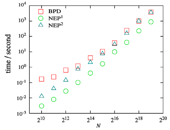
Fig. 4 (Color online) The computation time of two stages (the BPD and NEP algorithms) in the fast NBA on ER graph with $\langle k\rangle=3.0$ and nodes number from $N=2^{10}$ to $2^{19}$ (Intel Xeon E5450, 3.00 GHz, 2 GB memory). |
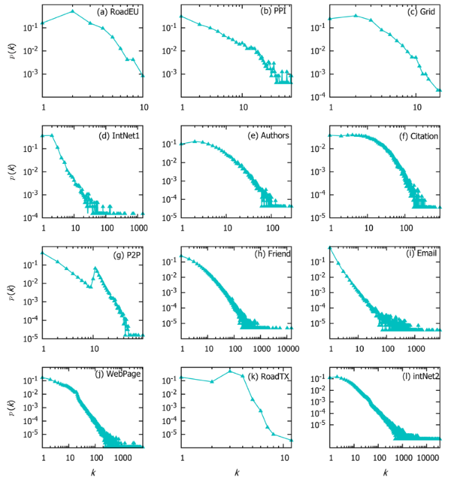
At last, we apply the fast NBA to dismantle some real-world networks, which contain plenty of communities, local loops, and hierarchical levels. We list the value of $R$ of the BPD algorithm and that of the fast ${\rm{NBA}^1}$ and fast ${\rm{NBA}^2}$ in Table 1. The fast NBA improves the general efficiency of the BPD remarkably from $r=8.0%$ (fast ${\rm{NBA}^1}$ in the Citation network) to $r=81.9%$ (fast ${\rm{NBA}^1}$ in the RoadTX network). Different from the case of the random graph ensembles, for the real-world networks, the fast ${\rm{NBA}^1}$ seems to be more suitable for reordering the dismantling sequence than fast ${\rm{NBA}^2}$. Although the fast ${\rm{NBA}^1}$ has a better general efficiency than fast ${\rm{NBA}^2}$ only in 7 of 12 real-world networks, which is not an overwhelming number, the average relative improvement of the fast ${\rm{NBA}^1}$ $\overline{r}=30.1%$ is almost twice of fast ${\rm{NBA}^2}$ $\overline{r}=17.2%$. The degree distributions of these real-world networks in Fig. 5 show that these networks contain the feature of the SF graph more or less.
Fig. 5 (Color online) The degree distribution of all real-world networks discussed in the Table 1. |
Table 1 Comparative results of the BPD algorithm, the fast ${\rm{NBA}^1}$ and fast ${\rm{NBA}^2}$ on twelve real-world networks. The number of nodes and edges of these networks are listed in the 2nd and 3rd column. The 4th column is the average degree of these networks. The general efficiency $R$ of the BPD algorithm, the fast ${\rm{NBA}^1}$ and fast ${\rm{NBA}^2}$ are listed in the 5th, 6th, and 7th column, correspondingly. We use boldface to highlight the minimum $R$ in the three algorithms. The relative improvement of the fast ${\rm{NBA}^1}$ and fast ${\rm{NBA}^2}$, denoted as $r^1$ and $r^2$ in the table, are listed in the 8th and 9th column, respectively. |
| Networks | BPD | fast NBA1 | fast NBA2 | r1 | r2 |
|---|---|---|---|---|---|
| RoadEU[32] * | 0.0455 | 0.0195 | 0.0418 | 0.57 | 0.08 |
| PPI[33] | 0.0923 | 0.0789 | 0.0809 | 0.14 | 0.12 |
| Grid[34] | 0.0355 | 0.0097 | 0.0298 | 0.73 | 0.16 |
| IntNet1[35] | 0.0123 | 0.0092 | 0.0104 | 0.25 | 0.15 |
| Authors[36] | 0.0877 | 0.0763 | 0.0755 | 0.13 | 0.14 |
| Citation[35] | 0.293 | 0.2695 | 0.2601 | 0.08 | 0.11 |
| P2P[35] | 0.1155 | 0.1047 | 0.1038 | 0.08 | 0.11 |
| Friend[35] | 0.1028 | 0.0918 | 0.0893 | 0.11 | 0.13 |
| Email[36] | 0.0013 | 0.0008 | 0.0008 | 0.35 | 0.36 |
| WebPage[37] | 0.0494 | 0.0410 | 0.0433 | 0.17 | 0.13 |
| RoadTX[37] | 0.0127 | 0.0023 | 0.0070 | 0.82 | 0.45 |
| intNet2[35] | 0.0372 | 0.0308 | 0.0321 | 0.17 | 0.14 |
The results in Fig. 2 also reveal that the fast ${\rm{NBA}^1}$ is better than fast ${\rm{NBA}^2}$ in extremely sparse SF graph. The RoadEU, Grid and RoadTX networks, where the fast ${\rm{NBA}^1}$ overwhelms fast ${\rm{NBA}^2}$, share a common feature that the average degree of them are very small ($\langle k\rangle<3$) and there is no node with massive connections. We believe that is one of the reasons why fast ${\rm{NBA}^1}$ is more fit for dismantling the three networks. The reader may argue that the average degree of the Email network is also smaller than $3$, but the two NBA algorithms give similar results. The reason is both fast NBA algorithms give a very small $R\approx 0.0008$, which is also the smallest one in all real-world networks and the fast ${\rm{NBA}^1}$ cannot behave better than fast ${\rm{NBA}^2}$ because the dismantling sequence given by the latter is already very close to the global optimum.
4 Conclusion
Many classical dismantling strategies, including the BPD algorithm, the Min-Sum algorithm, the equal graph partitioning algorithm, etc. focus on finding the minimum separate set while ignore the general efficiency of the removing order. The purpose of this paper is to further improve the general efficiency of an existed dismantling algorithm. We take the BPD algorithm as an example and explain how to use NPE algorithm to reorder the first $T$ nodes in the dismantling sequence given by the BPD. The BPD algorithm is good at giving a very small separate set and the NEP algorithm is more efficient during the dismantling process. The combination of the two algorithms gives birth to the NBA with the merit of both of them. Large-scale numerical computations on ER, RR, and SF graphs and twelve real-world networks reveal that although the NBA gives a dismantling threshold $\rho_c$ as small as or a little larger than that of the BPD, it greatly improves the general efficiency of the BPD algorithm. An algorithm compromising the best general efficiency and limited computation resources is introduced by setting $T=N\rho_c^{\rm{BPD}}$, which keeps the same computation complexity with the BPD.
Following the similar lines, we can also apply the framework of this kind of solution to other classical algorithms, such as the Min-Sum algorithm, the equal graph partitioning algorithm, etc. As long as we can find proper split points, the new algorithm will inherit multiple advantages from all ancestor algorithms and will not be in a higher complexity class than the slowest ancestor algorithm.