


1 Introduction
Many social, biological, and physical phenomena can be well understood on the top of complex networks.[1-6] A common topic in the research community is to establish the relationship between the topologies and the dynamics on them. Owing to degree heterogeneity in the interacting patterns, many fascinating phenomena have been revealed, such as the anomalous scaling behavior of Ising model,[7-11] a vanishing percolation threshold,[12-13] the absence of epidemic thresholds that separate healthy and endemic phases[14-16] and explosive emergence of phase transitions.[17-30]
The heterogeneous mean-field (HMF) theory has been widely used to study dynamical processes on complex networks.[3,5-6] This theory is based on the assumption that the nodes of the same degree are statistically equivalent. The main purpose of the HMF theory is to derive the dynamical equations for the quantities of interest in different degree classes. In general, the set of dynamical equations are intertwined with each other. However, for degree uncorrelated networks, they can be reduced to a single equation for an order parameter, such as the average magnetization in the Ising model[8] and the average infection probability in the susceptible-infected-susceptible model.[14] By linear stability analysis near the phase transition point, the HMF theory can produce an elegant analytical result of the phase transition point. For example, it has been shown that the critical temperature of the Ising model is $T_c=\langle {k^2} \rangle / \langle {k} \rangle $,[8] where $\langle {k^n} \rangle$ is the $n$th moment of degree distribution $P(k)$. For scale-free networks, $P(k) \sim k ^{-\gamma}$ with the exponent $\gamma<3$, $\langle {k^2} \rangle$ is divergent, and thus $T_c \rightarrow \infty$. The HMF theory has also shown its power in many other models, such as rumor spreading model,[31-32] metapopulation model,[33] zero-temperature Ising model,[34-35] majority-vote model,[36-37] etc.
In the present work, we propose an improved heterogenous mean-field (IHMF) theory to study the Ising model on complex networks. We derive the mean-field equation and then obtain the critical condition under which the phase transition temperature should be satisfied. Under the approximation of large average degree, the phase transition temperature $T_c$ is given analytically, $T_c = {{\langle {{k^2}} \rangle }}/{{\langle k \rangle }} - {{\langle k \rangle \langle {{k^3}} \rangle }}/{{{{\langle {{k^2}} \rangle }^2}}}$, that is different from the result of the HMF theory, ${{\langle {{k^2}} \rangle }}/{{\langle k \rangle }}$. By extensive Monte Carlo simulations in diverse types of networks, we find that our theoretical result is more successful in predicting $T_c$ than the previous HMF theory.
2 Model and Simulation Details
The Ising model in a network of size $N$ is described by the Hamiltonian,
$$ E = - J\sum\limits_{i < j} {{A_{ij}}{\sigma _i}{\sigma _j}}\,, $$
where spin variable $\sigma_i$ at node $i$ takes either $+1$ (up) or $-1$ (down). $J>0$ is the ferrimagnetic interaction constant. The elements of the adjacency matrix of the network take $A_{ij}=1$ if nodes $i$ and $j$ are connected and $A_{ij}=0$ otherwise.
The Monte Carlo (MC) simulation is performed by the so-called Glauber spin-flip dynamics,[38] in which one attempts to flip each spin once, on average, during each MC cycle. In each attempt, a randomly chosen spin $i$ is tried to flip with the probability
$$ {w_i}= \frac{1}{2}\Big[ {1 - \tanh \Big( {\frac{{\beta \Delta E}}{2}} \Big)} \Big]\,, $$
where $\beta=1/(k_B T)$ is the inverse temperature, $k_B$ is the Boltzmann constant, and $\Delta E = 2{\sigma _i}\sum\nolimits_j {{A_{ij}}{\sigma _j}}$ is the energy change due to the flipping process.
3 Theoretical Results
Let us define $m_k$ as the average magnetization of a node of degree $k$, i.e., ${m_k} = N_k^{ - 1}\sum\nolimits_{i,{k_i} = k}^{} {{\sigma _i}}$, where $N_k$ is the number of nodes of degree $k$. For a network without degree correlation, the probability of an end node of a randomly chosen edge having connectivity $k$ is $k$P($k$)/${{\langle k \rangle }}$,[3] where $P(k)=N_k/N$ is the probability of a randomly chosen node having connectivity $k$, and $\langle k \rangle = \sum\nolimits_{k'} {k'} P({k'})$ is the average degree. Thus, the average magnetization of an end node of a randomly chosen edge can be written as,
$$ tilde m = \sum\limits_{k} {\frac{{k P(k)}}{{\langle k\rangle }}} {m_{k}}\,. $$
This implies that the spin orientation of an end node of a randomly chosen edge points up or down with the probability $(1+\tilde m)/2$ or $(1-\tilde m)/2$, respectively. Thus, for a node of degree $k$, the probability that there are $n$ up spins among the neighborhood of the node can be written as a binomial distribution
$$ {p_{k,n}(\tilde m)} = C_k^n {\Big( {\frac{{1 + \tilde m}}{2}}\Big)^n}{\Big( {\frac{{1 - \tilde m}}{2}} \Big)^{k -n}}\,, $$
where $C_k^n = k!/[n!(k-n)!]$ is the binomial coefficient. For an up-spin node of degree $k$ with $n$ up-spin neighbor, the energy change to flip this spin is $4n-2k$. Combining Eqs. (2) and (4), we can write down the probability of flipping an up-spin node of degree $k$,
$$ w_k^ + = \frac{1}{2} - \frac{1}{2}\sum\limits_{n = 0}^k {{p_{k,n}}}\tanh ( {\beta ( {2n - k} )} )\,. $$
Likewise, we can express the probability of flipping a down-spin node of degree $k$ as
$$ w_k^ - = \frac{1}{2} + \frac{1}{2}\sum\limits_{n = 0}^k {{p_{k,n}}}\tanh ( {\beta ( {2n - k} )} )\,. $$
At each spin-flip process, the expectation of the change in $m_k$ can be written as
$$ \Delta {m_k} =\frac{{{N_k}}}{N}\Big( { - \frac{2}{{{N_k}}}}\Big)\Big( {\frac{{1 + {m_k}}}{2}} \Big)w_k^ +\\\ +\frac{{{N_k}}}{N}\Big( { + \frac{2}{{{N_k}}}} \Big)\Big({\frac{{1 - {m_k}}}{2}} \Big)w_k^ -\,, $$
where the factor is $N_k/N$ which is the probability that a class of nodes of degree $k$ are chosen, and $\mp 2/N_k$ is the change in $m_k$ due to the flip of an up (down) spin of degree $k$, and $(1 \pm m_k)/2$ is the probability of an up (down) spin of degree $k$ is chosen. If we set $\Delta t=1/N$, Eq. (7) can be rewritten as
$$ \frac{{d{m_k}}}{{d t}} = - ( {1 + {m_k}} )w_k^ + + ( {1 - {m_k}} )w_k^ - {\frac{{d{m_k}}}{{d t}} }= - {m_k} + \sum\limits_{n = 0}^k {{p_{k,n}(\tilde m)}} \tanh [ {\beta ( {2n - k} )} ]\,. $$
Substituting Eq. ({3}) into Eq. ({8}), we arrive at a self-consistent equation of $\tilde m$,
$$ \frac{{d\tilde m}}{{d t}} = - \tilde m + \sum\limits_k {\frac{{kP(k)}}{{\langle k \rangle }}} \sum\limits_{n = 0}^k{{p_{k,n}(\tilde m)}} \tanh [ {\beta ( {2n - k} )}]\,. $$
In equilibrium, $d \tilde m/d t=0$ and $d m_k/d t=0$, we have
$$ \tilde m = \sum\limits_k{\frac{{k P(k)}}{{\langle k \rangle }}} \sum\limits_{n =0}^k {{p_{k,n}(\tilde m)}} \tanh [ {\beta ( {2n - k})} ]\,, $$
$$ {m_k}= \sum\limits_{n = 0}^k {{p_{k,n}(\tilde m)}} \tanh [ {\beta ( {2n - k} )} ]\,. $$
Considering the fact
$ p_{k,n}(0)= p_{k,k-n}(0)\,, \quad \tanh (-x) = -\tanh (x)\,,$
it is not hard to verify that $\tilde m=0$ is always a solution of Eq. ({10}). Such a trivial solution corresponds to a disordered phase. The other solutions corresponding to $\tilde m\neq 0$ (an ordered phase) exist when the solution of $\tilde m=0$ loses its stability. This requires that the derivative of the right hand side of Eq. ({10}) with respect to $\tilde m$ is larger than one at $\tilde m=0$. The requirement yields the critical temperature of the Ising model that separates the disorder phase and ordered phase. To the end, we expand $p_{k,n}$ around $\tilde m=0$ to the first order, $ {p_{k,n}(\tilde m)} = p_{k,n}(0) + p_{k,n}(0) ( {2n - k} )\tilde m + O(\tilde m^2) $ with ${p_{k,n}}(0) = C_k^n{(1/ 2)^k}$.)^k}$. The critical temperature is determined by
$$ {\sum\limits_k {\frac{{k P(k)}}{{\langle k \rangle }}\sum\limits_{n = 0}^k {{p_{k,n}}(0)(2n - k)\tanh[ {\beta_c(2n - k)} ]} } = 1\,.}$$
Equation (12) is the main result of the present work. For a given degree distribution $P(k)$, the critical temperature $T_c=1/\beta_c$ can be calculated numerically by Eq. ({12}). Moreover, for networks with large average degree, $\beta_c$ approaches to zero. To the end, we expanse
$$ \tanh( {{\beta _c}(2n - k)} ) \approx {\beta _c}(2n - k)- \frac{1}{3}\beta _c^3{(2n - k)^3}\,, $$
and substitute Eq. ({13}) into Eq. ({12}), we have
$$ \sum\limits_k {\frac{{k P(k)}}{{\langle k \rangle }}}\Big[ {\langle {{{(2n - k)}^2}} \rangle {\beta _c} -\frac{1}{3}\langle {{{(2n - k)}^4}} \rangle \beta _c^3}\Big] = 1\,, $$
where
$$ \langle {{{(2n - k)}^2}} \rangle = \sum\limits_{n = 0}^k{{p_{k,n}}(0){{(2n - k)}^2}} = k\,, $$
$$ \langle {{{(2n - k)}^4}} \rangle = \sum\limits_{n = 0}^k{{p_{k,n}}(0){{(2n - k)}^4}} = k(3 k-2)\approx 3k^2\,. $$
Substituting Eqs. ({15}) and ({16}) into Eq. ({14}), we obtain
$$ \frac{{\langle {{k^2}} \rangle }}{{\langle k\rangle }}{\beta _c} - \frac{{\langle {{k^3}}\rangle }}{{\langle k \rangle }}\beta _c^3 =1\,, $$
where $\langle {{k^n}} \rangle = \sum\nolimits_k{{k^n}P(k)}$ is the $n$-th moment of degree distribution.
If we drop out the second term on the left hand side of Eq. (17), we recover to the result of the HMF theory,
$$ T_c^{\rm HMF} = \frac{{\langle {{k^2}} \rangle}}{{\langle k \rangle }}\,. $$
Substituting Eq. (18) into Eq. (17), we arrive at an improved result of the HMF theory,
$$ T_c^{\rm IHMF} = \frac{{\langle {{k^2}} \rangle}}{{\langle k \rangle }} - \frac{{\langle k\rangle \langle {{k^3}} \rangle }}{{{{\langle{{k^2}} \rangle }^2}}}\,. $$
4 Numerical Validation
In order to validate the theoretical result, we need to numerically determine $T_c$, which can be located by calculating the so-called Binder's fourth-order cumulant $U$,[39] defined as
$$ U = 1 - \frac{{[ {\langle {{m^4}} \rangle }]}}{{3{{[ {\langle {{m^2}} \rangle }]}^2}}}\,, $$
where $m = \sum_{i = 1}^N {{\sigma _i}}/N$ is the average magnetization per node, $\langle \cdot \rangle$ denotes time averages taken at equilibrium, and $[ \cdot ]$ stands for the averages over different network configurations for a given degree distribution. $T_c$ is estimated as the point where the curves $U \sim T$ for different network sizes $N$ intercept each other.
We first show the results in regular random networks (RRNs), in which each node is randomly connected to exactly $k$ neighbors and degree distribution follows the $\delta$-function, and thus $\langle {{k^n}} \rangle = {k^n}$,
$$ T_{c,\rm RRN}^{\rm HMF} = k\,, $$
$$ T_{c,\rm RRN}^{\rm IHMF} = k - 1\,.$$
In Fig. 1(a), we show $U$ as a function of $T$ for different network sizes $N$ in RRNs with $k=4$. The intersection point locates the critical temperature $T_c=2.88$, which is closer to our theoretical result $k-1=3$ (Eq. (22)) than the previous one $k=4$ (Eq. (21)). In Fig. 1(b), we compare the numerical results of $T_c$ with the theoretical predictions for different $k$'s in RRNs. It is obvious that our improved theory is superior to the previous HMF theory.
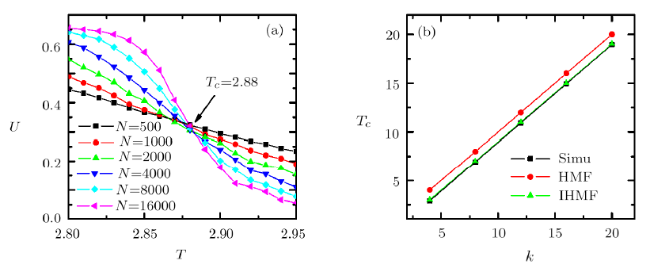
Fig. 1 (Color online) (a) The Binder's fourth-order cumulant $U$ as a function of the temperature $T$ for different network sizes $N$ in RRNs with $k=4$. (b) The critical temperature $T_c$ in RRNs as a function of $k$. |
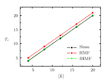
Fig. 2 (Color online) The critical temperature $T_c$ in ER random networks as a function of average degree $\langle k\rangle$. |
For Erd\"os-Rényi (ER) random networks whose degree distribution follows a Poisson distribution,$P(k) = e^{-\langle k \rangle } {\langle k \rangle }^k/ {k!}$, we have $\langle {{k^2}} \rangle = {\langle k \rangle^2} + \langle k \rangle$ and $\langle {{k^3}}\rangle = {\langle k \rangle ^3} + 3{\langle k \rangle ^2} + \langle k \rangle$,
$$ T_{c,\rm ER}^{\rm HMF} = \langle k \rangle + 1\,, $$
$$ T_{c,\rm ER}^{\rm IHMF} = \langle k \rangle -\frac{{\langle k \rangle }}{{{{( {\langle k \rangle + 1} )}^2}}} \approx \langle k \rangle\,. $$
In Fig. 2, we compare the numerical results of $T_c$ with the theoretical predictions for different average degree $\langle k \rangle$ in ER random networks. As expected, our improved theory is superior to the previous HMF theory.
For scale-free networks (SFNs) whose degree distribution follows a power-law function,
$P(k) = ( {\gamma - 1} )k_0^{\gamma- 1}{k^{ - \gamma }}\,,$
with the minimal degree $k_0$ and the power exponent of degree distribution $\gamma$, we have $\langle k\rangle=( {\gamma - 1} ){k_0}/({\gamma - 2})$,$\langle k^2 \rangle=( {\gamma - 1} ){k_0^2}/({\gamma - 3)}$,$\langle k^3 \rangle=( {\gamma - 1} ){k_0^3}/({\gamma - 4})$
$$ T_{c,\rm SF}^{\rm HMF} = \frac{{\gamma - 2}}{{\gamma -3}}{k_0}\,, $$
$$ T_{c,\rm SF}^{\rm IHMF} = \frac{{\gamma - 2}}{{\gamma - 3}}{k_0} -\frac{{{{( {\gamma - 3} )}^2}}}{{( {\gamma - 2})( {\gamma - 4} )}}\,. $$
As mentioned before, for SFNs with $\gamma \leq 3$, $\langle k^2 \rangle$ is divergent in the limit of $N \rightarrow \infty$, and thus $T_c \rightarrow \infty$. While for $3<\gamma\leq4$, $\langle k^3 \rangle$ is divergent in the limit of $N \rightarrow \infty$, and therefore Eq. ({26}) is only valid for $\gamma>4$. In Fig. 3(a) and 3(b), we show the results in SFNs with $\gamma=4.5$ and $\gamma=5.0$,respectively. It is obvious that our improved theory is more inagreement with the simulation results than the previous HMF theory.
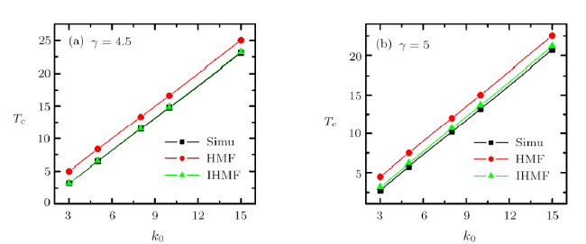
Fig. 3 (Color online) The critical temperature $T_c$ in SF networks as a function of minimal degree $k_0$. (a) $\gamma=4.5$;(b) $\gamma=5$. |
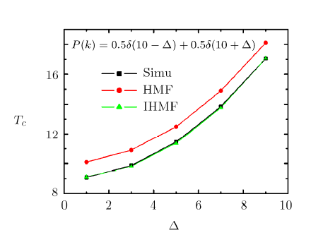
Fig. 4 (Color online) The critical temperature $T_c$ in random networks with a bimodal degree distribution $P(k) =({1}/{2})\delta ( {k - \langle k \rangle - \Delta} ) + ({1}/{2})\delta ( {k - \langle k \rangle + \Delta } )$ with $\langle k\rangle=10$. |
At last, we construct a network with degree distribution following a bimodal distribution $P(k) = ({1}/{2})\delta ( {k -\langle k \rangle - \Delta } ) + ({1}/{2})\delta( {k - \langle k \rangle + \Delta } )$. We have $\langle k \rangle = \langle k \rangle$,$\langle {{k^2}} \rangle = {\langle k \rangle^2} + {\Delta ^2}$, and $\langle {{k^3}} \rangle = {\langle k \rangle^3} + 3{\Delta^2}\langle k \rangle$. In terms of Eqs. ({18}) and ({19}), we can obtain the results of the HMF and IHMF theories. As shown in Fig. 4, the IHMF theory is more accurate in predicting the critical temperature than the HMF theory.
5 Conclusions
In conclusion, we have proposed an improved heterogeneous mean-field theory to study the Ising model on complex networks. Our theory shows that the critical temperature of the Ising model is $T_c=\langle k^2 \rangle/\langle k \rangle -\langle k \rangle \langle k^3 \rangle/\langle k^2 \rangle ^2$, that is an improvement of the result of the customary heterogeneous mean-field theory, $\langle k^2 \rangle/\langle k \rangle$. By comparing the critical temperature with simulations in various networks, we have shown that our theoretical prediction is more accurate than the previous heterogeneous mean-field one.