This paper focuses on the issue of resilient dynamic output-feedback (DOF) control for ${{ \mathcal H }}_{\infty }$ synchronization of chaotic Hopfield networks with time-varying delay. The aim is to determine a DOF controller with gain perturbations ensuring that the ${{ \mathcal H }}_{\infty }$ norm from the external disturbances to the synchronization error is less than or equal to a prescribed bound. A delay-dependent criterion for the ${{ \mathcal H }}_{\infty }$ synchronization is derived by employing the Lyapunov functional method together with some recent inequalities. Then, with the help of some decoupling techniques, sufficient conditions on the existence of the resilient DOF controller are developed for both the time-varying and constant time-delay cases. Lastly, an example is used to illustrate the applicability of the results obtained.
Xin Huang(黄鑫), Youmei Zhou(周幼美), Qingkai Kong(孔庆凯), Jianping Zhou(周建平), Muyun Fang(方木云). ${{ \mathcal H }}_{\infty }$ synchronization of chaotic Hopfield networks with time-varying delay: a resilient DOF control approach*[J]. Communications in Theoretical Physics, 2020, 72(1): 015003. DOI: 10.1088/1572-9494/ab5452
1. Introduction
Hopfield network, a type of interconnected artificial neural network introduced by John J. Hopfield in 1982 [1], provides an innovative model for understanding and imitating memory in the human brain. Over the last two decades, there is a growing interest in the study of dynamic behaviors of Hopfield networks owing to the fact that they are closely related to many applications such as combinatorial optimization [2], content-addressable memory [3], and blind signal detection [4]. In [5], a Hopfield network with symmetric connection weight matrix was considered. It was proved therein that the network is absolute stable if and only if the weight matrix is negative semi-definite. When one is faced with the problem of asymmetric weight matrix, some sufficient conditions for global asymptotic stability were reported in [6]. A qualitative Hopf bifurcation analysis of a Hopfield network consisting of four neurons was given in [7], where the features of the limit cycles related to the bifurcations were acquired with the aid of normal forms theory. Periodic oscillation of discrete Hopfield networks was discussed [8], where several criteria for the uniqueness and exponential stability of oscillatory solutions were derived by utilizing coincidence degree theory. In [9], the chaotic regime of a six-neuron Hopfield network was analyzed, and it was demonstrated that many attractors can be obtained under appropriate choices of the network parameters.
The results in the above references rely on the assumption that the neurons can communicate and respond to each other instantaneously, which is questionable in hardware implementation due to the limited switching speed of amplifiers. In [10], a constant time delay was first introduced into the continuous-time Hopfield networks. It was shown that, for a certain type of connection topology, even a small delay may affect the system performance seriously. Later, multiple constant time delays were introduced in [11] to reflect different communication channels. And when the time delay was allowed to be time-varying, the existing criteria of almost periodic solutions were proposed in [12], while sufficient conditions for global asymptotic or even global exponential stability were given in [13]. It is now well recognized that the introduction of time delays into a Hopfield network can greatly enrich the dynamic behavior of the network. In particular, it has been shown that time-delay Hopfield networks are able to generate a large variety of strange chaotic attractors including single-scroll chaotic attractors [14], double-scroll chaotic attractors [15], three-chaos and periodic four-torus attractors [16], etc. Correspondingly, much attention has been paid to synchronization design of chaotic time-delay Hopfield networks in recent years in view of its potential application in secure communication, and some valid control schemes have been adopted; see, e.g., [17] for the adaptive control scheme and [18] for the memory control scheme.
One of the most important issues in control theory is how to construct controllers with acceptable performance in the presence of exogenous disturbances. Generally, one has no prior knowledge of the statistics of the disturbances. This situation has led to the development of ${{ \mathcal H }}_{\infty }$ control in the past several decades as such a control strategy offers many advantages, especially the insensitive property to the disturbance statistics [19–21]. For chaotic neural networks with time delay, the problem of exponential ${{ \mathcal H }}_{\infty }$ synchronization control was considered in [22] and [23] in continuous-time and discrete-time respectively, where some sufficient conditions on the existence of delayed state-feedback controllers were presented. In [24], a delay-dependent ${{ \mathcal H }}_{\infty }$ synchronization control scheme was developed in terms of linear matrix inequalities (LMIs). In the context of packet dropouts, sampled-data ${{ \mathcal H }}_{\infty }$ synchronization control strategies were designed in [25] by employing the Lyapunov functional theory. It should be noted that, although there are a number of studies on ${{ \mathcal H }}_{\infty }$ synchronization control of chaotic time-delay neural networks available in the literature, most of them are founded on full state feedback, which requires that all neuron states should be available. In practice, a complete measurement of the neuron states may be hard, costly, and even infeasible to implement. In this situation, the output-feedback control strategy is more preferable for engineering applications as the outputs of a system are generally easier to obtain than the states [26–29].
Motivated by the above analysis, in the present study, we focus on the design of resilient dynamic output-feedback (DOF) controller for ${{ \mathcal H }}_{\infty }$ synchronization of a class of chaotic Hopfield networks with time-varying delay. The time-delay function is supposed to be continuous and bounded, but not necessarily differentiable. Our purpose is to determine a DOF controller with gain perturbations ensuring the ${{ \mathcal H }}_{\infty }$ norm from the external disturbances to the synchronization error is less than or equal to a prescribed bound (called the ${{ \mathcal H }}_{\infty }$ disturbance attenuation bound). The issue of resilient DOF controller design is non-convex in nature and remains challenging. By selecting a proper Lyapunov functional together with using the Wirtinger inequality and the reciprocally convex combination lemma, we derive a delay-dependent criterion for ${{ \mathcal H }}_{\infty }$ synchronization. For the constant time delay case, a delay-dependent ${{ \mathcal H }}_{\infty }$ synchronization condition is also proposed. On the basis of the criteria and with the help of some decoupling techniques, we develop sufficient conditions on the existence of the resilient DOF controller for both the time-varying and constant time-delay cases. It is worth mentioning that the desired controller gain can be obtained through the feasible solution of a few LMIs, which is easy to solve by the well-known mathematical software Matlab. Lastly, we give an example to illustrate the applicability of the results obtained.
Let ${{\mathbb{R}}}^{p}$ be the p-dimensional Euclidean space, ${{\mathbb{R}}}^{p\times q}$ be the group of p × q real matrices, and ${{\mathbb{S}}}^{p}$ (respectively, ${{\mathbb{S}}}_{+}^{p}$) be the group of real symmetric square matrices (respectively, real symmetric positive-definite square matrices) of order p. In a symmetric matrix, the blocks that can be obviously inferred by symmetry are represented by $\ast $. Let Ip and 0p be the p-order unit matrix and zero matrix, respectively. The notation $\parallel \cdot \parallel $ refers to the Euclidean vector norm, $\mathrm{diag}\{\cdot \cdot \cdot \}$ denotes a diagonal matrix, MT denotes the transpose of matrix M, and He(M) stands for M + MT.
2. Preliminaries
Let us consider a neural network with dynamic model:
where $x(t)\in {{\mathbb{R}}}^{{n}_{1}}\ $ is the neuron state; $y(t)\in {{\mathbb{R}}}^{m}$ represents the output; $A,{A}_{\tau },B,{B}_{\tau },C$ are constant real matrices; $J\in {{\mathbb{R}}}^{{n}_{1}}$ denotes a constant input; $f(\cdot )\in {{\mathbb{R}}}^{{n}_{1}}$ and $g(\cdot )\in {{\mathbb{R}}}^{{n}_{1}}$ are two activation functions that both are global Lipschitz continuous [30–32]; i.e., there are Lipschitz constants Lf and Lg such that
for any ${\delta }_{1},{\delta }_{2}\in {{\mathbb{R}}}^{{n}_{1}}$. One can refer to [33, 34] for more relaxed activation functions. τ (t) stands for the time delay that is continuous and belonging to a given interval as [35]:
where τ1 and τ2 are known constants. Note that the time delay is time-varying, which is more general than the constant time delay discussed in [36, 37]. It is also worth mentioning that, unlike that commonly used in the literature (see, e.g., [38–42]), the time-varying delay considered herein is not required to be differentiable with respect to t.
The response system under consideration is given as follows:
where $\hat{x}(t)\in {{\mathbb{R}}}^{{n}_{1}}$ and $\hat{y}(t)\in {{\mathbb{R}}}^{{n}_{1}}$ are, respectively, the state and the output; $u(t)\in {{\mathbb{R}}}^{{n}_{1}}$ and $\omega (t)\in {{\mathbb{R}}}^{k}$ denote, respectively, the control input and the external disturbance belonging to ${{ \mathcal L }}_{2}[0,\infty );$$D\in {{\mathbb{R}}}^{{n}_{1}\times k}$ is a constant real matrix. Define $e(\cdot )=\hat{x}(\cdot )-x(\cdot )$. Then one is able to establish the following error system
In (8), ${e}_{K}(t)\in {{\mathbb{R}}}^{{n}_{c}}$ denotes the state of the controller, ${A}_{K},{B}_{K},{C}_{K},{D}_{K}$ are the controller gains to be determined later, and ${\rm{\Delta }}{A}_{K},{\rm{\Delta }}{B}_{K}$, ${\rm{\Delta }}{C}_{K},{\rm{\Delta }}{D}_{K}$ stand for the gain perturbations, which are assumed to be norm-bounded as [43, 44]:
where M, N are constant real matrices, and F is an uncertain matrix satisfying ${F}^{{\rm{T}}}F\leqslant I$. It is worth mentioning that the resilient DOF controller to be designed is of full-order when nc = n1 and of reduced-order when nc < n1. Particulary, when nc = 0, the controller reduces to the usual static output-feedback controller.
Although there are many results on ${{ \mathcal H }}_{\infty }$ synchronization control of chaotic time-delay neural networks available in the literature, only a few of them consider the robustness of controllers. Due to the rounding error of digital computing, the restriction of process memory, and the noise of analog-digital conversion, it is often the case that the designed controllers possess parameter inaccuracies to some degree, and even a tiny perturbation to the controller gain may greatly undermine the controller’s performance [45–48]. Thus the design of resilient controller is of practical importance.
Combining (6) with (7), we get
$ \begin{eqnarray}\begin{array}{rcl}\dot{\xi }(t) & = & {{ \mathcal A }}_{K}\xi (t)+{{ \mathcal A }}_{\tau }\xi \left(t-\tau (t,)\right)+{ \mathcal B }\bar{f}\left(\xi (t,)\right)\\ & & +{{ \mathcal B }}_{\tau }\bar{g}\left(\xi \left(t-\tau (t\right),)\right)+{ \mathcal D }\omega (t),\end{array}\end{eqnarray}$
Before ending the section, we recall the definition of ${{ \mathcal H }}_{\infty }$ synchronization and prepare some lemmas that are needed for establishing our main results.
([49] ${{ \mathcal H }}_{\infty }$ synchronization).Error system (6) is called ${{ \mathcal H }}_{\infty }$ synchronized, if, under the zero initial condition,
holds for a pre-defined level $\gamma \gt 0$ (called the ${{ \mathcal H }}_{\infty }$ disturbance attenuation bound), where ${Q}_{1}$ is a positive symmetric matrix.
([50] Improved Wirtinger’s inequality).For a specific matrix $R\in {{\mathbb{S}}}_{+}^{n}$ and any function $\eta $ that is differentiable in $\left[p,q\right]\to {{\mathbb{R}}}^{n}$, one has
regarding a real scalar $\rho \gt 0$ and real matrices ${\rm{\Lambda }},{U}_{i},{V}_{i}$ and ${W}_{i}(i=1,\,\cdots ,\,N)$ is satisfied. Then one can write
3. ${{ \mathcal H }}_{\infty }$ synchronization analysis
This section focuses on the ${{ \mathcal H }}_{\infty }$ synchronization analysis for the error system. A sufficient condition is given by the following theorem:
For given scalar $\gamma \gt 0$ and ${Q}_{1}$ in ${{\mathbb{S}}}_{+}^{{n}_{1}}$, system (6) is ${{ \mathcal H }}_{\infty }$ synchronized, if there are scalars ${\varepsilon }_{f}\gt 0,{\varepsilon }_{g}\gt 0$ and matrices $P$ in ${{\mathbb{S}}}_{+}^{3n},{S}_{1},{S}_{2},{R}_{1},{R}_{2}$ in ${{\mathbb{S}}}_{+}^{n},{N}_{1},$${N}_{2}$ in ${R}^{9n\times 2n}$ such that
$ \begin{eqnarray*}{\rm{\Xi }}=\left[\begin{array}{cc}{{\rm{\Phi }}}_{0}(\beta )-{\rm{\Theta }}(\beta ) & {G}_{1}^{{\rm{T}}}(\beta )P\tilde{D}+{g}_{0}^{{\rm{T}}}({\tau }_{1}^{2}{R}_{1}+{\tau }_{12}^{2}{R}_{2}){ \mathcal D }\\ * & {{ \mathcal D }}^{{\rm{T}}}({\tau }_{1}^{2}{R}_{1}+{\tau }_{12}^{2}{R}_{2}){ \mathcal D }-{\gamma }^{2}I\end{array}\right].\end{eqnarray*}$
If ${\rm{\Xi }}\lt 0$ holds for $\beta =\tfrac{\tau (t)-{\tau }_{1}}{{\tau }_{12}}$, then one can get ${J}_{t}\lt 0$ for any ${\left[\begin{array}{cc}{\zeta }^{{\rm{T}}}(t) & {\omega }^{{\rm{T}}}(t)\end{array}\right]}^{{\rm{T}}}\ne 0$, which means
and, thus system (6) is ${{ \mathcal H }}_{\infty }$ synchronized in the sense of definition 1.
From the above analysis, now one just need to show that inequality ${\rm{\Xi }}\lt 0$ can be guaranteed by the condition of this Theorem. In fact, by Schur’s complement one can rewrite ${\rm{\Xi }}\lt 0$ as
$ \begin{eqnarray*}{\rm{\Phi }}(\beta )={{\rm{\Phi }}}_{0}(\beta )-\phi {\left({{ \mathcal D }}^{{\rm{T}}}({\tau }_{1}^{2}{R}_{1}+{\tau }_{12}^{2}{R}_{2}){ \mathcal D }-{\gamma }^{2}I\right)}^{-1}{\phi }^{{\rm{T}}}\end{eqnarray*}$
with
$ \begin{eqnarray*}\phi ={G}_{1}^{{\rm{T}}}(\beta )P\tilde{D}+{g}_{0}^{{\rm{T}}}({\tau }_{1}^{2}{R}_{1}+{\tau }_{12}^{2}{R}_{2}){ \mathcal D }.\end{eqnarray*}$
Since Φ (β) is quadratic with respect to β, one can see that Φ (β) is convex function. Then, using lemma 3, (23) holds for any $\beta =\tfrac{\tau (t)-{\tau }_{1}}{{\tau }_{12}}\in (0,\ 1)$ if
is satisfied for all β$=\,\left\{0,1\right\}$. Using Schur’s complement again, (24) can be rewritten as (13) with α replaced by β. Thus, the proof is completed.□
By utilizing augmented LKF (14) together with the improved Wirtinger’s inequality and the generalized reciprocally convex combination lemma, a delay-dependent condition for the ${{ \mathcal H }}_{\infty }$ synchronization of error system (6) is derived without the requirement of differentiability of the delay function. From the proof, it is not difficult to see that the condition also ensures the asymptotical stability of error system (6).
When the time delay is constant (i.e., τ(t) = τ), augmented system (10) turns to
$ \begin{eqnarray}\begin{array}{rcl}\dot{\xi }(t) & = & {{ \mathcal A }}_{K}\xi (t)+{{ \mathcal A }}_{\tau }\xi \left(t-\tau \right)+{ \mathcal B }\bar{f}\left(\xi (t,)\right)\\ & & +{{ \mathcal B }}_{\tau }\bar{g}\left(\xi \left(t-\tau \right)\right)+{ \mathcal D }\omega (t).\end{array}\end{eqnarray}$
In this situation, one can establish the following theorem:
For given scalar $\gamma \gt 0,Q$ in ${{\mathbb{S}}}_{+}^{n}$, system (6) with constant time delay is ${{ \mathcal H }}_{\infty }$ synchronized, if there are scalars ${\varepsilon }_{f}\gt 0,{\varepsilon }_{g}\gt 0$ and matrices $P$ in ${{\mathbb{S}}}_{+}^{2n},{S}_{1},{R}_{1}$ in ${{\mathbb{S}}}_{+}^{n}$ such that
$ \begin{eqnarray}\left[\begin{array}{cc}{{\rm{\Phi }}}_{0} & {G}_{1}^{{\rm{T}}}P\tilde{D}+{\tau }^{2}{g}_{0}^{{\rm{T}}}{R}_{1}{ \mathcal D }\\ * & {\tau }^{2}{{ \mathcal D }}^{{\rm{T}}}{R}_{1}{ \mathcal D }-{\gamma }^{2}I\end{array}\right]\lt 0,\end{eqnarray}$
$ \begin{eqnarray*}\begin{array}{l}\dot{V}({\xi }_{t},{\dot{\xi }}_{t})={\left[\begin{array}{c}\zeta (t)\\ \omega (t)\end{array}\right]}^{{\rm{T}}}\\ \times \,\left[\begin{array}{cc}{{\rm{\Phi }}}_{0}-\mathrm{diag}(Q,{0}_{4n}) & {G}_{1}^{{\rm{T}}}P\tilde{D}+{\tau }^{2}{g}_{0}^{{\rm{T}}}{R}_{1}{ \mathcal D }\\ * & {\tau }^{2}{{ \mathcal D }}^{{\rm{T}}}{R}_{1}{ \mathcal D }\end{array}\right]\left[\begin{array}{c}\zeta (t)\\ \omega (t)\end{array}\right].\end{array}\end{eqnarray*}$
Then, along similar lines as those in the proof of theorem 1, one can easily show that system (6) with constant time delay is ${{ \mathcal H }}_{\infty }$ synchronized. The reminder is omitted for brevity.□
4. ${{ \mathcal H }}_{\infty }$ synchronization synthesis
This section focuses on the design of resilient DOF controller to ensure the ${{ \mathcal H }}_{\infty }$ synchronization of the error system. A constructive approach is presented by the following theorem:
For given scalars $\gamma \gt 0$ , $\rho \gt 0$, resilient DOF controller (7) ensures the ${{ \mathcal H }}_{\infty }$ synchronization of drive system (1) and response system (5), if there exist scalars $\varepsilon \gt 0,{\varepsilon }_{f}\gt 0,{\varepsilon }_{g}\gt 0$, and matrices $P={({P}_{{ij}})}_{3\times 3}$ in ${{\mathbb{S}}}_{+}^{3n},{S}_{1},{S}_{2},{R}_{1},{R}_{2}$ in ${{\mathbb{S}}}_{+}^{n},{N}_{1},{N}_{2}$ in ${R}^{9n\times 2n},X,Y$ such that the following LMI holds true
which, together with lemma 2, implies (37). In this way, the proof is completed.□
For the situation of constant time delay, the following result can be established via following similar lines as those in the derivation of theorem 3:
For given scalars $\gamma \gt 0$ , $\rho \gt 0$, resilient DOF controller (7) ensures the ${{ \mathcal H }}_{\infty }$ synchronization of drive system (1) and response system (5) with constant time delay, if there exist scalars $\varepsilon \gt 0,{\varepsilon }_{f}\gt 0,{\varepsilon }_{g}\gt 0$, and matrices $P={({P}_{{ij}})}_{2\times 2}$ in ${{\mathbb{S}}}_{+}^{2n},{S}_{1},{R}_{1}$ in ${{\mathbb{S}}}_{+}^{n},X,Y$ such that the following LMI
$ \begin{eqnarray*}\begin{array}{rcl}{G}_{01} & = & \left[\begin{array}{ccccc}\tilde{A} & {{ \mathcal A }}_{\tau } & 0 & { \mathcal B } & {{ \mathcal B }}_{\tau }\\ I & -I & 0 & 0 & 0\end{array}\right],\ {g}_{01}=\left[\begin{array}{ccccc}\tilde{A} & {{ \mathcal A }}_{\tau } & 0 & { \mathcal B } & {{ \mathcal B }}_{\tau }\end{array}\right],\\ {{\rm{\Delta }}}_{1} & = & {P}_{11}\tilde{B},\ {{\rm{\Delta }}}_{3}=\tau {P}_{12}^{{\rm{T}}}\tilde{B},\ {{\rm{\Delta }}}_{6}={\tau }^{2}{{ \mathcal D }}^{{\rm{T}}}{R}_{1}\tilde{B},\ {{\rm{\Delta }}}_{7}={\tau }^{2}{R}_{1}\tilde{B},\end{array}\end{eqnarray*}$
where ${\tilde{S}}_{{fg}}$ and ${G}_{2}$ are the same as those in theorem 2. In this case, the desired gain is given by (34).
With the help of lemma 2 and Schur’s complement, theorems 3 and 4 give sufficient conditions on the existence of resilient DOF controller (7) for ensuring the ${{ \mathcal H }}_{\infty }$ synchronization of drive system (1) and response system (5) with time-varying delay and constant delay, respectively. These conditions possess the form of LMIs and, hence, are able to be easily checked via the well-known mathematical software Matlab. Once the LMI conditions are feasible, the desired control gain can be obtained by (34).
5. Simulation examples
In the section, an example is applied to show the applicability of the presented DOF ${{ \mathcal H }}_{\infty }$ synchronization control approaches.
Consider a time-delay Hopfield neural network as follows:
where Mi and Ni ($i=1,\,\cdots ,\,{n}_{1}+{n}_{c}$) are random numbers belonging to $(-3,3)$. Then, theorem 3 can be utilized to seek the resilient DOF controller (7) ensuring the ${{ \mathcal H }}_{\infty }$ synchronization of the drive-response systems. Especially, when taking ρ = 0.1 and τ1 = 0.5, the minimum allowed ${{ \mathcal H }}_{\infty }$ disturbance attenuation bound for different (nc, τ2) is given in table 1, from which one can see the designed resilient DOF controller of different orders yields different results.
Thus, according to theorem 3, the ${{ \mathcal H }}_{\infty }$ synchronization of the drive-response systems can be ensured by the designed resilient DOF controller with gain $K={X}^{-1}Y$.
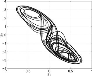
Suppose that $\omega (t)={\left[5{e}^{-2t},3{e}^{-2t}\right]}^{{\rm{T}}}$ and
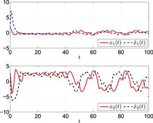
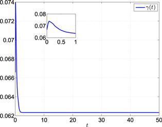
Then, the phase-plane trajectories of the drive system and unforced response system are shown in figures 1 and 2, respectively. The state trajectories are depicted in figure 3. One can observe that both the drive and unforced response systems have chaotic behaviors, and they are not synchronized even under the same initial condition. Let us change the initial condition of the response system to be $\left[{\hat{x}}_{1}(s),{\hat{x}}_{2}(s)\right]\,=[-1.2,\ -3.0],\ s\in [-1,0]$. Then, under the designed resilient DOF controller, the plot of
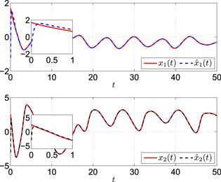
and the state trajectories of the drive-response systems are shown in figures 4 and 5, respectively. It can be seen that γ (t) < γ = 0.1084 and the chaos synchronization of the drive-response systems is achieved very quickly.
Figure 5. State trajectories with control when nc = 1.
6. Conclusion
In this paper, a resilient DOF controller for ${{ \mathcal H }}_{\infty }$ synchronization of a class of chaotic Hopfield networks with the time-varying delay has been designed. By employing the Lyapunov functional method together with some recent inequalities, a delay-dependent criterion for the ${{ \mathcal H }}_{\infty }$ synchronization has been derived. Then, with the help of some decoupling techniques, sufficient conditions for the existence of the resilient DOF controller have been developed for both the time-varying and constant time-delay cases.
HopfieldJ J1982 Neural networks and physical systems with emergent collective computational abilities Proc. of the National Academy of Sciences79 2554 2558
FortiMManettiSMariniM1994 Necessary and sufficient condition for absolute stability of neural networks IEEE Transactions on Circuits and Systems I: Fundamental Theory and Applications41 491 494
SongXSongSBalseraI TLiuL2017 Mixed ${{ \mathcal H }}_{\infty }$ and passive projective synchronization for fractional order memristor-based neural networks with time-delay and parameter uncertainty Commun. Theor. Phys.68 483 494
LiYWangHMengX2019 Almost automorphic synchronization of quaternion-valued high-order Hopfield neural networks with time-varying and distributed delays IMA J. Math. Control Inf.36 983 1013
ZhouJWangYZhengXWangZShenH2019 Weighted ${{ \mathcal H }}_{\infty }$ consensus design for stochastic multi-agent systems subject to external disturbances and ADT switching topologies Nonlinear Dyn.96 853 868
WangJRuTXiaJWeiYWangZ2019 Finite-time synchronization for complex dynamic networks with semi-Markov switching topologies: an ${{ \mathcal H }}_{\infty }$ event-triggered control scheme Appl. Math. Comput.356 235 251
KarimiH RGaoH2010 New delay-dependent exponential ${{ \mathcal H }}_{\infty }$ synchronization for uncertain neural networks with mixed time delays IEEE Transactions on Systems, Man, and Cybernetics, Part B40 173 185
QiDLiuMQiuMZhangS2010 Exponential ${{ \mathcal H }}_{\infty }$ synchronization of general discrete-time chaotic neural networks with or without time delays IEEE Trans. Neural Networks21 1358 1365
ChangXLiuRParkJ H2019 A further study on output feedback ${{ \mathcal H }}_{\infty }$ control for discrete-time systems IEEE Trans. Circuits Syst. Express Briefs (in press)
YanZSangCFangMZhouJ2018 Energy-to-peak consensus for multi-agent systems with stochastic disturbances and Markovian switching topologies Trans. Inst. Meas. Control40 4358 4368
LiXZhouCZhouJWangZXiaJ2019 Couple-group ${{ \mathcal L }}_{2}-{{ \mathcal L }}_{\infty }$ consensus of nonlinear multi-agent systems with Markovian switching topologies Int. J. Control Autom. Syst.17 575 585
FanYHuangXLiYXiaJChenG2019 Aperiodically intermittent control for quasi-synchronization of delayed memristive neural networks: an interval matrix and matrix measure combined method IEEE Transactions on Systems, Man, and Cybernetics: Systems49 2254 2265
YanZZhouYHuangXZhouJ2019 Finite-time boundedness for time-delay neural networks with external disturbances via weight learning approaches Mod. Phys. Lett. B33 1950343
YanZHuangXCaoJ2019 Variable-sampling-period dependent global stabilization of delayed memristive neural networks via refined switching event-triggered control Sci. China Inf. Sci. (in press)
CaoYSamiduraiRSriramanR2019 Robust passivity analysis for uncertain neural networks with leakage delay and additive time-varying delays by using general activation function Math. Comput. Simul.155 57 77
ZhouJSangCLiXFangMWangZ2018 ${{ \mathcal H }}_{\infty }$ consensus for nonlinear stochastic multi-agent systems with time delay Appl. Math. Comput.325 41 58
ZhuangGMaQZhangBXuSXiaJ2018 Admissibility and stabilization of stochastic singular Markovian jump systems with time delays Systems & Control Letters114 1 10
ZhuangGXuSXiaJMaQZhangZ2019 Non-fragile delay feedback control for neutral stochastic Markovian jump systems with time-varying delays Appl. Math. Comput.355 21 32
WangFYangHZhangSHanF2016 Containment control for first-order multi-agent systems with time-varying delays and uncertain topologies Commun. Theor. Phys.66 249 255
ShiKWangJZhongSZhangXLiuYChengJ2019 New reliable nonuniform sampling control for uncertain chaotic neural networks under Markov switching topologies Appl. Math. Comput.347 169 193
WangZShenLXiaJShenHWangJ2018 Finite-time non-fragile ${l}_{2}-{l}_{\infty }$ control for jumping stochastic systems subject to input constraints via an event-triggered mechanism J. Franklin Inst.355 6371 6389
XiaJGaoHLiuMZhuangGZhangB2018 Non-fragile finite-time extended dissipative control for a class of uncertain discrete time switched linear systems J. Franklin Inst.355 3031 3049
SeuretAGouaisbautFFridmanE2013 Stability of systems with fast-varying delay using improved Wirtinger’s inequality 2013 IEEE 52nd Annual Conf. on Decision and Control 946 951


