


1. Introduction
The nonlinear interaction of several wave modes has attracted great interest, and particular attention has been focused on the (2 + 1)-dimensional three-wave equation [1–10] and the three-dimensional three-wave equation [11–14]. These equations can be applied to the problems of radiophysics and nonlinear optics [15]. Besides the continuous integrable system, the consideration of integrable discretization or discrete integrable equations is also important. To our knowledge, the references about (2 + 1)-dimensional discrete three-wave equation are few.
The feasible approach based on the $\bar{\partial }$ (Dbar)-problem [16–23] is a powerful tool to investigate the integrability of nonlinear PDEs, in particular for higher dimensional equations, and to find their explicit solutions, including soliton solutions. In addition, The Dbar-problem also provides a method to construct the symmetry conditions of integrable equations [24].
Extending the Zakharov–Shabat dressing method is one of the important methods to form and solve discrete integrable nonlinear equations [24–26]. Here, in this paper, we extend the Dbar-dressing method to investigate the discrete (2 + 1)-dimensional differential-difference equation $ \begin{eqnarray}\begin{array}{l}{\rm{i}}{\partial }_{t}[{a}_{q}{Q}_{{pq}}(n)-{a}_{p}{Q}_{{pq}}(n-1)]\\ \qquad -\,{\rm{i}}{\partial }_{y}[{b}_{q}{Q}_{{pq}}(n)-{b}_{p}{Q}_{{pq}}(n-1)]\\ \quad =\,{s}_{{pq}}[{R}_{p}(n){Q}_{{pq}}(n)-{Q}_{{pq}}(n-1){R}_{q}(n)]\\ \qquad +\,{s}_{{pq}}(1-{E}^{-}){Q}_{{pq}}(n)-{s}_{{pq}}{Q}_{{pr}}(n-1){Q}_{{rq}}(n)\\ \qquad +\,{s}_{{rq}}{Q}_{{pr}}(n){Q}_{{rq}}(n)+{s}_{{pr}}{Q}_{{pr}}(n-1){Q}_{{rq}}(n-1),\\ \quad r\ne p\ne q,\end{array}\end{eqnarray}$ $ \begin{eqnarray}\begin{array}{l}(1-{E}^{-})[{{\rm{i}}{a}}_{p}{\partial }_{t}{Q}_{{pp}}(n)-{\rm{i}}{\partial }_{y}{Q}_{{pp}}(n)\\ \quad -\,\displaystyle \sum _{r\ne p}{s}_{{pr}}| {Q}_{{pr}}(n){| }^{2}]=0,\end{array}\end{eqnarray}$ where ${E}^{-}$ is the backward shift, and aq, bq, (q = 1, 2, 3) are real constants and $ \begin{eqnarray}{R}_{p}(n)={Q}_{{pp}}(n)-{Q}_{{pp}}(n-1),\quad {s}_{{pq}}={b}_{p}{a}_{q}-{a}_{p}{b}_{q}.\end{eqnarray}$ Here and after, we have omitted the dependence of the variables y and t.
Let us impose the following constraint ${Q}^{\dagger }(n)=-Q(n)$ with $Q(n)={\left({Q}_{{pq}}(n\right)}_{3\times 3}$ , which implies that Qpp(n) is purely imaginary. Here † denotes the Hermitian conjugate. It is noted that equations (1.1 ) and (1.2 ) were derived through the discrete version of Zakharov–Shabat dressing method [25]. We note that the linear equation (1.2 ) can be rewritten as a forced equation $ \begin{eqnarray}\begin{array}{c}\begin{array}{l}{\rm{i}}{ \mathcal L }\left(\begin{array}{c}{Q}_{11}(n)\\ {Q}_{22}(n)\\ {Q}_{33}(n)\end{array}\right)\,=\,S\left(\begin{array}{c}| {Q}_{12}(n){| }^{2}\\ | {Q}_{13}(n){| }^{2}\\ | {Q}_{23}(n){| }^{2}\end{array}\right)\,+\,F,\\ S=\left(\begin{array}{ccc}{s}_{12} & {s}_{13} & 0\\ -{s}_{12} & 0 & {s}_{23}\\ 0 & -{s}_{13} & -{s}_{23}\end{array}\right),\\ { \mathcal L }={\rm{diag}}(\begin{array}{c}{a}_{1}{{\rm{\partial }}}_{t}-{b}_{1}{{\rm{\partial }}}_{y},{a}_{2}{{\rm{\partial }}}_{t}-{b}_{2}{{\rm{\partial }}}_{y},{a}_{3}{{\rm{\partial }}}_{t}-{b}_{3}{{\rm{\partial }}}_{y},\end{array}),\\ F={\left({f}_{1},{f}_{2},{f}_{3}\right)}^{{\rm{T}}},\,detS=0.\end{array}\end{array}\,\end{eqnarray}$ Here fp, (p = 1, 2, 3) are real functions and are independent of the variable n. In addition, equation (1.4 ) implies the forced conservation law $ \begin{eqnarray}{{\rm{\partial }}}_{t}\left(\displaystyle \sum _{p=1}^{3}{{\rm{i}}a}_{p}{Q}_{{pp}}(n)\right)-{{\rm{\partial }}}_{y}\left(\displaystyle \sum _{p=1}^{3}{{\rm{i}}b}_{p}{Q}_{{pp}}(n)\right)=\displaystyle \sum _{p=1}^{3}{f}_{p},\end{eqnarray}$ and Qpp(n) is representation of the energy functions $| {Q}_{{pq}}(n){| }^{2},$ (1 ≤ p < q ≤ 3) by virtue of $\det S=0$ . More concisely, in the case of fp = 0, Qpp(n) is determined only by the energy functions $| {Q}_{{pq}}{| }^{2}$ and $| {Q}_{{pr}}{| }^{2}$ in view of (1.4 ), where $p\ne q\ne r$ . The total energy ${\sum }_{p=1}^{3}{{\rm{i}}a}_{p}{\int }_{-\infty }^{\infty }{Q}_{{pp}}(n){\rm{d}}y$ is conserved, if ${Q}_{{pp}}(n)\to 0$ as $| y| \to \infty $ . Hence, equations (1.1 ) and (1.2 ) model a forced (2 + 1)-dimensional discrete three-wave (FD3W) equation.
In the paper, two covariant derivative operators and one backward translation operator are introduce to construct the Lax pair of the FD3W equation. A suitable symmetry condition is found to derive the soliton solutions. It is remarked that forces fp in (1.4 ) are zero for soliton solutions. We have to say that the picture of the forces to solution is not yet clear.
The whole paper is organized as follows. In section 2 , the dressing method is presented to derive the Lax pair of the FD3W equation. In section 3 , the nonlocal Dbar-problem and the symmetry condition are introduced. In section 4 , the explicit solutions in several cases are given. In section 5 , we give brief remarks about another form of FD3W equation and its soliton solution derived from another symmetry constraint.
2. Dressing approach
Given two diagonal constant matrices A and B, we consider the following covariant derivatives $ \begin{eqnarray}\begin{array}{c}\begin{array}{rcl}{{\bf{D}}}_{t}\chi & = & {\rm{i}}{\chi }_{t}+k\chi B,\,\,\,B={\rm{diag}}({b}_{1},{b}_{2},{b}_{3}),\\ {{\bf{D}}}_{y}\chi & = & {\rm{i}}{\chi }_{y}+k\chi A,\,\,\,A={\rm{diag}}({a}_{1},{a}_{2},{a}_{3}),\end{array}\end{array}\end{eqnarray}$ and the backward translation operator $ \begin{eqnarray}{\bf{T}}\chi =({E}^{-}\chi )(1-k)I,\end{eqnarray}$ where I is the unit matrix and ${E}^{\pm }$ is the shift operator ${E}^{\pm }\chi (n)=\chi (n\pm 1)$ . Here χ = χ(n, y, t; k) and k is the complex spectral parameter.
Suppose χ has the following asymptotic behavior $ \begin{eqnarray}\chi =I+{k}^{-1}{\chi }^{(1)}+{k}^{-2}{\chi }^{(2)}\,+\,\cdots ,\quad k\to \infty ,\end{eqnarray}$ where ${\chi }^{(j)}={\chi }^{(j)}(n,y,t)$ is independent of k. Introduce two new functions $ \begin{eqnarray}\begin{array}{rcl}v(n) & = & {BQ}(n-1)-Q(n)B,\\ u(n) & = & {AQ}(n-1)-Q(n)A,\end{array}\end{eqnarray}$ where $ \begin{eqnarray}Q(n)={\chi }^{(1)}(n).\end{eqnarray}$ Here we omit the variables y, t for convenience. After a regularization procedure, we find the following linear system $ \begin{eqnarray}\begin{array}{rcl}{{\bf{D}}}_{t}\chi +B({\bf{T}}\chi )-B\chi +v(n)\chi & = & 0,\\ {{\bf{D}}}_{y}\chi +A({\bf{T}}\chi )-A\chi +u(n)\chi & = & 0,\end{array}\end{eqnarray}$ or $ \begin{eqnarray}\begin{array}{c}\begin{array}{l}{\rm{i}}{\chi }_{t}+k\chi B+B({E}^{-}\chi )(1-k)\\ \,-\,B\chi +(Q(n)B-{BQ}(n-1))\chi =0,\\ {\rm{i}}{\chi }_{y}+k\chi A+A({E}^{-}\chi )(1-k)\\ \,-\,A\chi +(Q(n)A-{AQ}(n-1))\chi =0.\end{array}\end{array}\end{eqnarray}$ Substituting (2.3 ) into (2.7 ), the term of $O({k}^{-1})$ of system (2.7 ) implies $ \begin{eqnarray}\begin{array}{c}\begin{array}{l}{{\rm{i}}Q}_{y}(n)+{\chi }^{(2)}(n)A-A{\chi }^{(2)}(n-1)\\ \,+\,A[Q(n-1)-Q(n)]+u(n)Q(n)=0,\\ {{\rm{i}}Q}_{t}(n)+{\chi }^{(2)}(n)B-B{\chi }^{(2)}(n-1)\\ \,+\,B[Q(n-1)-Q(n)]+v(n)Q(n)=0,\end{array}\end{array}\end{eqnarray}$ in terms of (2.5 ). Consider the derivative of u(n) in (2.4 ) with respect to t and v(n) with respect to y, and eliminate χ(2) by subtracting the results, we arrive at $ \begin{eqnarray}\begin{array}{c}\begin{array}{l}{{\rm{i}}u}_{t}(n)-{{\rm{i}}v}_{y}(n)\\ \,=\,A({E}^{+}-1)Q(n-1)B-B({E}^{+}-1)Q(n-1)A\\ \,+\,{BQ}(n-1)Q(n)A-{AQ}(n-1)Q(n)B\\ \,+\,Q(n)[{AQ}(n)B-{BQ}(n)A]\\ \,+\,[{AQ}(n-1)B-{BQ}(n-1)A]Q(n-1).\end{array}\end{array}\end{eqnarray}$ The elements of equation (2.9 ) give rise to the FD3W equations (1.1 ) and (1.2 ).
3. Dbar-problem and symmetry condition
To obtain the solution of the FD3W equations (1.1 ) and (1.2 ), we introduce the following nonlocal Dbar-problem $ \begin{eqnarray}\bar{\partial }\chi (k,\bar{k})=\iint \chi (z,\bar{z})R(z,\bar{z};k,\bar{k}){\rm{d}}z\wedge {\rm{d}}\bar{z},\end{eqnarray}$ with canonical normalization condition, where $R(z,\bar{z};k,\bar{k})$ is the spectral transformation matrix. This problem is equivalent to the following integral equation $ \begin{eqnarray}\begin{array}{l}\chi (k,\bar{k})=I+\displaystyle \frac{1}{2\pi {\rm{i}}}\iint \displaystyle \frac{{\rm{d}}\mu \wedge {\rm{d}}\bar{\mu }}{\mu -k}\\ \quad \times \iint \chi (\lambda ,\bar{\lambda })R(\lambda ,\bar{\lambda };\mu ,\bar{\mu }){\rm{d}}\lambda \wedge {\rm{d}}\bar{\lambda }.\end{array}\end{eqnarray}$ Here and after, we take the domain to be the entire complex plane.
For the FD3W equations (1.1 ) and (1.2 ), if χ is a solution of the Dbar-problem (3.1 ), one needs to introduce the variables n, y, t into the spectral transformation matrix and take $ \begin{eqnarray}\begin{array}{l}R(z,\bar{z};k,\bar{k};n,y,t)\\ \quad =\,{\psi }_{0}(z;n,y,t){R}_{0}(z,\bar{z};k,\bar{k}){\psi }_{0}^{-1}(k;n,y,t),\end{array}\end{eqnarray}$ where $ \begin{eqnarray}{\psi }_{0}(k;n,y,t)=\displaystyle \frac{1}{{\left(1-k\right)}^{n}}\exp \{-{\rm{i}}k\theta \},\,\theta ={Ay}+{Bt},\end{eqnarray}$ satisfies the following condition $ \begin{eqnarray}{\psi }_{0}^{\dagger }(\bar{k};n,y,t)=\displaystyle \frac{1}{{\left(1-k\right)}^{2n}}{\psi }_{0}^{-1}(k;n,y,t).\end{eqnarray}$ Here ${R}_{0}(z,\bar{z};k,\bar{k})$ is independent of the variables n, y, t and satisfies the following symmetry condition [24] $ \begin{eqnarray}{\left(\displaystyle \frac{1-k}{1-z}\right)}^{2n}{R}_{0}^{\dagger }(\bar{z},z;k,\bar{k})={R}_{0}(k,\bar{k};z,\bar{z}).\end{eqnarray}$
4. Explicit solutions
Substituting (2.3 ) into (3.2 ), we get the representation of χ(1)(n, y, t) $ \begin{eqnarray}\begin{array}{rcl}{\chi }^{(1)}(n,y,t) & = & -\displaystyle \frac{1}{2\pi {\rm{i}}}\iint {\rm{d}}\mu \wedge {\rm{d}}\bar{\mu }\\ & & \times \iint \chi (\lambda ,\bar{\lambda })R(\lambda ,\bar{\lambda };\mu ,\bar{\mu };n,y,t){\rm{d}}\lambda \wedge {\rm{d}}\bar{\lambda }.\end{array}\end{eqnarray}$ If the spectral transformation matrix is degenerate and takes the following form $ \begin{eqnarray}R(\lambda ,\bar{\lambda };\mu ,\bar{\mu };n,y,t)=\displaystyle \sum _{j=1}^{N}{f}_{j}(\lambda ,\bar{\lambda };n,y,t){g}_{j}(\mu ,\bar{\mu };n,y,t),\end{eqnarray}$ then we have $ \begin{eqnarray}{\chi }^{(1)}(n,y,t)=-\displaystyle \frac{1}{2\pi {\rm{i}}}\hat{\xi }{\left(I+M\right)}^{-1}\check{\eta },\end{eqnarray}$ where $\hat{\xi }=({\xi }_{1},{\xi }_{2},\,\cdots ,\,{\xi }_{N}),\check{\eta }=\left(\begin{array}{c}{\eta }_{1}\\ \vdots \\ {\eta }_{N}\end{array}\right)$ and $M={({M}_{{jl}})}_{(3N)\times (3N)}$ , $ \begin{eqnarray}\begin{array}{c}\begin{array}{rcl}{\xi }_{j} & = & \iint {f}_{j}(\lambda ,\bar{\lambda };n,y,t){\rm{d}}\lambda \wedge {\rm{d}}\bar{\lambda },\\ {\eta }_{j} & = & \iint {g}_{j}(\mu ,\bar{\mu };n,y,t){\rm{d}}\mu \wedge {\rm{d}}\bar{\mu },\\ {M}_{{jl}} & = & \displaystyle \frac{1}{2\pi {\rm{i}}}\iint \iint \displaystyle \frac{{g}_{j}(\mu ,\bar{\mu };n,y,t){f}_{l}(\lambda ,\bar{\lambda };n,y,t)}{\lambda -\mu }\\ & & \times {\rm{d}}\bar{\mu }\wedge {\rm{d}}\mu {\rm{d}}\bar{\lambda }\wedge {\rm{d}}\lambda .\end{array}\end{array}\end{eqnarray}$
Furthermore, if set
$ \begin{eqnarray*}\begin{array}{rcl}{f}_{j}(\lambda ,\bar{\lambda };n,y,t) & = & {\psi }_{0}(\lambda ;n,y,t){f}_{j0}(\lambda ,\bar{\lambda }),\\ {g}_{j}(\mu ,\bar{\mu };n,y,t) & = & {g}_{j0}(\mu ,\bar{\mu }){\psi }_{0}^{-1}(\mu ;n,y,t),\end{array}\end{eqnarray*}$
then we have
$ \begin{eqnarray}{f}_{j0}(\lambda ,\bar{\lambda })={\left(1-\lambda \right)}^{2n}{g}_{j0}^{\dagger }(\bar{\lambda },\lambda ).\end{eqnarray}$ in terms of the symmetry condition (3.6 ).
then we have
To obtain the soliton solutions of the FD3W equations (1.1 ) and (1.2 ), we first choose $ \begin{eqnarray}\begin{array}{c}\begin{array}{rcl}{g}_{j}(\mu ,\bar{\mu };n,y,t) & = & {C}_{j}\exp \{{\rm{i}}\mu \theta \}{\left(1-\mu \right)}^{n}\delta (\mu -{k}_{j}),\\ {f}_{j}(\lambda ,\bar{\lambda };n,y,t) & = & \exp \{-{\rm{i}}\lambda \theta \}{C}_{j}^{\dagger }{\left(1-\lambda \right)}^{n}\delta (\lambda -{\bar{k}}_{j}),\end{array}\end{array}\end{eqnarray}$ where θ is defined in (3.4 ) and Cj is a constant matrix. Substituting (4.6 ) into (4.4 ), we obtain $ \begin{eqnarray}{\xi }_{j}=-{{\rm{i}}Z}_{j}^{\dagger },\,{\eta }_{j}=-{{\rm{i}}Z}_{j},\,{M}_{{jl}}=\displaystyle \frac{1}{2\pi {\rm{i}}}\displaystyle \frac{{Z}_{j}{Z}_{l}^{\dagger }}{{k}_{j}-{\bar{k}}_{l}},\end{eqnarray}$ where $ \begin{eqnarray}{Z}_{j}=2{C}_{j}{\left(1-{k}_{j}\right)}^{n}\exp \{{{\rm{i}}k}_{j}\theta \}.\end{eqnarray}$ Note that ${\xi }_{j}=-{\eta }_{j}^{\dagger }$ and ${M}_{{lj}}^{\dagger }={M}_{{jl}}$ , which imply that ${{\chi }^{(1)}}^{\dagger }=-{\chi }^{(1)}$ in view of (4.3 ).
In general, if choose the element of matrix gj and fj as $ \begin{eqnarray}\begin{array}{c}\begin{array}{rcl}{g}_{j}^{({pq})}(\mu ,\bar{\mu };n,y,t) & = & {C}_{j}^{({pq})}{{\rm{e}}}^{{\rm{i}}\mu {\theta }_{q}}{\left(1-\mu \right)}^{n}\delta (\mu -{k}_{j}^{({pq})}),\\ {f}_{j}^{({pq})}(\lambda ,\bar{\lambda };n,y,t) & = & {{\rm{e}}}^{-{\rm{i}}\lambda {\theta }_{p}}{\bar{C}}_{j}^{({qp})}{\left(1-\lambda \right)}^{n}\delta (\lambda -{\bar{k}}_{j}^{({qp})}),\end{array}\end{array}\,\end{eqnarray}$ then we have (p, q = 1, 2, 3) $ \begin{eqnarray}\begin{array}{c}\begin{array}{c}\begin{array}{rcl}{\eta }_{j}^{\left({pq}\right)} & = & -{{\rm{i}}Z}_{j}^{\left({pq}\right)},\,{\xi }_{j}^{\left({qp}\right)}=-{\rm{i}}{\bar{Z}}_{j}^{\left({qp}\right)},\\ {M}_{{jl}}^{\left({pq}\right)} & = & \displaystyle \frac{1}{2\pi {\rm{i}}}\displaystyle \sum _{r=1}^{3}\displaystyle \frac{{Z}_{j}^{\left({pr}\right)}{\bar{Z}}_{l}^{\left({qr}\right)}}{{k}_{j}^{\left({pr}\right)}-{\bar{k}}_{l}^{\left({qr}\right)}},\end{array}\end{array}\end{array}\end{eqnarray}$ where ${\theta }_{q}={a}_{q}y+{b}_{q}t$ and $ \begin{eqnarray}{Z}_{j}^{({pq})}=2{C}_{j}^{({pq})}{{\rm{e}}}^{{{\rm{i}}k}_{j}^{({pq})}{\theta }_{q}}{\left(1-{k}_{j}^{({pq})}\right)}^{n}.\end{eqnarray}$
Thus, in both case of (4.6 ) and (4.9 ), the solution of the FD3W equations (1.1 ) and (1.2 ) takes the form $ \begin{eqnarray}\begin{array}{c}Q=\displaystyle \frac{1}{2\pi {\rm{i}}}{\check{Z}}^{\dagger }{\left(I+M\right)}^{-1}\check{Z},\,\check{Z}={\left(\begin{array}{c}{Z}_{1}\\ \vdots \\ {Z}_{N}\end{array}\right)}_{(3N)\times 3}.\end{array}\end{eqnarray}$
Furthermore, the elements in qth column of the matrix Zj are ${Z}_{j}^{(* q)}$ , and the collection of these elements composes the qth column of the matrix $\check{Z}$ , denoted by ${\check{Z}}^{(q)}$ . Note that ${\check{Z}}^{(q)}$ is a (3N) × 1 matrix. Using these notations, the element of the solution Q can be rewritten as $ \begin{eqnarray}\begin{array}{l}{Q}_{{pq}}=-\displaystyle \frac{1}{2\pi {\rm{i}}}\displaystyle \frac{\det {\left(I+M\right)}_{{pq}}^{(a)}}{\det (I+M)},\\ {\left(I+M\right)}_{{pq}}^{(a)}=\left(\begin{array}{cc}0 & {\left({\check{Z}}^{(p)}\right)}^{\dagger }\\ {\check{Z}}^{(q)} & (I+M)\end{array}\right).\end{array}\end{eqnarray}$ We note that representation for higher-order solution can be found in [27, 28].
For the general case (4.9 ), If take $1-{k}_{j}^{({pq})}={{\rm{e}}}^{{\sigma }_{j}^{({pq})}+{\rm{i}}{\phi }_{j}^{({pq})}}$ , then ${k}_{j}^{({pq})}=1-{{\rm{e}}}^{{\sigma }_{j}^{({pq})}}\cos {\phi }_{j}^{({pq})}-{\rm{i}}{{\rm{e}}}^{{\sigma }_{j}^{({pq})}}\sin {\phi }_{j}^{({pq})}$ . In this case, ${Z}_{j}^{({pq})}$ in (4.11 ) can be denoted as $ \begin{eqnarray}\begin{array}{rcl}{Z}_{j}^{({pq})} & = & 2{{\rm{e}}}^{{X}_{j}^{({pq})}+{{\rm{i}}{T}}_{j}^{({pq})}},\\ {X}_{j}^{({pq})} & = & n{\sigma }_{j}^{({pq})}+{{\rm{e}}}^{{\sigma }_{j}^{({pq})}}\sin {\phi }_{j}^{({pq})}\cdot {\theta }_{q}+{X}_{j0}^{({pq})},\\ {T}_{j}^{({pq})} & = & n{\phi }_{j}^{({pq})}+(1-{{\rm{e}}}^{{\sigma }_{j}^{({pq})}}\cos {\phi }_{j}^{({pq})}){\theta }_{q}+{T}_{j0}^{({pq})}.\end{array}\end{eqnarray}$ Here we denote ${C}_{j}^{\left({pq}\right)}={{\rm{e}}}^{{X}_{j0}^{\left({pq}\right)}+{{\rm{i}}T}_{j0}^{\left({pq}\right)}}$ .
In particular, if we choose the constants ${C}_{j},(j=1,\,\cdots ,\,N)$ as row vectors, or ${C}_{j}=({C}_{j}^{(1)},{C}_{j}^{(2)},{C}_{j}^{(3)})$ . In this case, the elements of the row vector gj will be $ \begin{eqnarray}{g}_{j}^{(q)}={C}_{j}^{(q)}{\left(1-k\right)}^{n}{{\rm{e}}}^{{\rm{i}}k{\theta }_{q}}\delta (k-{k}_{j}^{(q)}),\,q\,=\,1,2,3,\end{eqnarray}$ which imply that the element ${Z}_{j}^{(q)}$ of the row vector Zj takes the same form as these in (4.14 ), but with the superscript (q) instead of (pq). In addition, the matrix M in (4.13 ) reduces to a N × N matrix, with element Mjl taking the following form $ \begin{eqnarray}\begin{array}{c}\begin{array}{l}{M}_{{jl}}=\displaystyle \frac{2}{{\rm{i}}\pi }\displaystyle \sum _{q=1}^{3}\displaystyle \frac{1}{{k}_{j}^{(q)}-{\bar{k}}_{l}^{(q)}}{{\rm{e}}}^{{\rm{i}}({T}_{j}^{(q)}-{T}_{l}^{(q)})}{{\rm{e}}}^{{X}_{j}^{(q)}+{X}_{l}^{(q)})},\\ \,(j,l=1,\,\cdots N),\end{array}\end{array}\end{eqnarray}$ Here ${X}_{j}^{(q)}$ and ${T}_{j}^{(q)}$ have the same definitions as those in (4.14 ), but with the superscript (q) instead of (pq). We note that the discrete spectrum ${k}_{j}^{(q)},(q=1,2,3)$ can not be real, because the diagonal part of the matrix M is undefined.
For N = 1, equation (4.13 ) reduces to the one soliton solution of the FD3W equations (1.1 ) and (1.2 ) $ \begin{eqnarray}{Q}_{{pq}}=\displaystyle \frac{2}{{\rm{i}}\pi }{{\rm{e}}}^{{\rm{i}}({T}_{1}^{(q)}-{T}_{1}^{(p)})}\displaystyle \frac{{{\rm{e}}}^{{X}_{1}^{(p)}+{X}_{1}^{(q)}}}{1\,+\,M},\,M=\displaystyle \frac{1}{\pi }\displaystyle \sum _{r=1}^{3}\displaystyle \frac{{{\rm{e}}}^{2{X}_{1}^{(r)}}}{{{\rm{e}}}^{{\sigma }_{1}^{(r)}}\sin {\phi }_{1}^{(r)}}.\end{eqnarray}$ Note that, for the soliton solution, the forces fp in (1.4 ) are zero.
If the imaginary part of the discrete spectrum admits ${\mathfrak{I}}({k}_{1}^{(q)})\gt 0,(q=1,2,3)$ , then $\sin ({\phi }_{1}^{(q)})\gt 0$ . Now we introduce the notations $ \begin{eqnarray}\begin{array}{rcl}{\tau }_{1}^{(q)} & = & \displaystyle \frac{1}{2}({\sigma }_{1}^{(q)}+\mathrm{ln}(\pi \sin ({\phi }_{1}^{(q)}))),\\ {\hat{X}}^{(q)} & = & {X}_{1}^{(q)}-{\tau }_{1}^{(q)},\quad q=1,2,3.\end{array}\end{eqnarray}$ The one soliton solution can be rewritten as $ \begin{eqnarray}{Q}_{{pq}}=\displaystyle \frac{1}{{\rm{i}}\pi }\displaystyle \frac{{{\rm{e}}}^{{\rm{i}}({T}_{1}^{(q)}-{T}_{1}^{(p)})}{{\rm{e}}}^{{X}^{(p)}+{X}^{(q)}}}{{{\rm{e}}}^{{\hat{X}}^{(p)}+{\hat{X}}^{(q)}}\cosh ({\hat{X}}^{(p)}-{\hat{X}}^{(q)})+{{\rm{e}}}^{{\hat{X}}^{(r)}}\cosh ({\hat{X}}^{(r)})},\end{eqnarray}$ and $ \begin{eqnarray}{Q}_{{qq}}=\displaystyle \frac{1}{{\rm{i}}\pi }\displaystyle \frac{{{\rm{e}}}^{2{X}^{(q)}}}{{{\rm{e}}}^{{\hat{X}}^{(r)}+{\hat{X}}^{(p)}}\cosh ({\hat{X}}^{(r)}-{\hat{X}}^{(p)})+{{\rm{e}}}^{{\hat{X}}^{(q)}}\cosh ({\hat{X}}^{(q)})},\end{eqnarray}$ where $1\leqslant p,q,r\leqslant 3$ and $r\ne p\ne q$ . Since the relationship between the two set solutions (1.4 ) are not simple, we still discuss them separately. In fact, the two set soliton solutions take different asymptotic analysis. In deed, along the ‘line’ ${\hat{X}}^{(p)}-{\hat{X}}^{(q)}=0$ , we find
$ \begin{eqnarray*}\begin{array}{c}\begin{array}{rcl}{Q}_{{pq}} & \to & \left\{\begin{array}{cl}0, & {\hat{X}}^{(r)}\to +\infty ,\\ \tfrac{{{\rm{\Omega }}}_{{pq}}}{{{\rm{e}}}^{-({\hat{X}}^{(p)}+{\hat{X}}^{(q)})}+2}, & {\hat{X}}^{(r)}\to -\infty ,\end{array}\right.\\ {Q}_{{rr}} & \to & \left\{\begin{array}{cl}{\rm{const}}, & {\hat{X}}^{(r)}\to +\infty ,\\ 0, & {\hat{X}}^{(r)}\to -\infty ,\end{array}\right.\end{array}\end{array}\end{eqnarray*}$
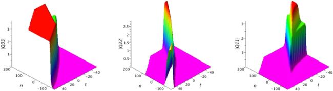
where$1\leqslant p\lt q\leqslant 3,1\leqslant r\leqslant 3$ and $r\ne p,q$ . Here ${{\rm{\Omega }}}_{{pq}}$ is a bounded function. If we further impose that ${\hat{X}}^{(p)}={\hat{X}}^{(q)}=c$ is a constant, then $| {Q}_{{pq}}| $ tends to a certain constant in the direction of ${\hat{X}}^{(r)}\to -\infty $ . Figure 1 shows the soliton solutions Qpq in (4.19 ) and figure 2 shows Qqq in (4.20 ).
where
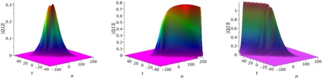
Figure 1. One-soliton solution Qpq at y = 0 in ( |
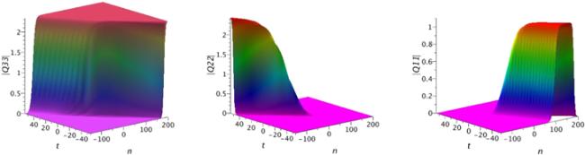
Figure 2. One-soliton solution Qqq at y = 0 in ( |
Similarly, if the discrete spectrum satisfies ${\mathfrak{I}}({k}_{1}^{(q)})\lt 0,(q=1,2,3)$ , or $\sin ({\phi }_{1}^{(q)})\lt 0$ . We introduce the notations $ \begin{eqnarray}\begin{array}{rcl}{\tilde{\tau }}_{1}^{(q)} & = & \displaystyle \frac{1}{2}({\sigma }_{1}^{(q)}+\mathrm{ln}(\pi | \sin ({\phi }_{1}^{(q)})| ),\\ {\tilde{X}}^{(q)} & = & {X}_{1}^{(q)}-{\tilde{\tau }}_{1}^{(q)},\quad q=1,2,3.\end{array}\end{eqnarray}$ We have another type of one soliton solution $ \begin{eqnarray}{Q}_{{pq}}=\displaystyle \frac{-1}{{\rm{i}}\pi }\displaystyle \frac{{{\rm{e}}}^{{\rm{i}}({T}_{1}^{(q)}-{T}_{1}^{(p)})}{{\rm{e}}}^{{X}^{(p)}+{X}^{(q)}}}{{{\rm{e}}}^{{\tilde{X}}^{(p)}+{\tilde{X}}^{(q)}}\cosh ({\tilde{X}}^{(p)}-{\tilde{X}}^{(q)})+{{\rm{e}}}^{{\tilde{X}}^{(r)}}\sinh ({\tilde{X}}^{(r)})},\end{eqnarray}$ and $ \begin{eqnarray}{Q}_{{qq}}=\displaystyle \frac{-1}{{\rm{i}}\pi }\displaystyle \frac{{{\rm{e}}}^{2{X}^{(q)}}}{{{\rm{e}}}^{{\tilde{X}}^{(r)}+{\tilde{X}}^{(p)}}\cosh ({\tilde{X}}^{(r)}-{\tilde{X}}^{(p)})+{{\rm{e}}}^{{\tilde{X}}^{(q)}}\sinh ({\tilde{X}}^{(q)})},\end{eqnarray}$ where $1\leqslant p,q,r\leqslant 3$ and $r\ne p\ne q$ . The asymptotic behaviors can be discussed similarly.
The other cases of the discrete spectrum can be discussed in the same way. For example, for $1\leqslant p,q,r\leqslant 3,p\lt q,{\mathfrak{I}}({k}_{1}^{(p)})\gt 0,{\mathfrak{I}}({k}_{1}^{(r)})\gt 0$ and ${\mathfrak{I}}({k}_{1}^{(q)})\lt 0$ , we have $ \begin{eqnarray}{Q}_{{pq}}=\displaystyle \frac{1}{{\rm{i}}\pi }\displaystyle \frac{{{\rm{e}}}^{{\rm{i}}({T}_{1}^{(q)}-{T}_{1}^{(p)})}{{\rm{e}}}^{{X}^{(p)}+{X}^{(q)}}}{{{\rm{e}}}^{{\hat{X}}^{(p)}+{\tilde{X}}^{(q)}}\sinh ({\hat{X}}^{(p)}-{\tilde{X}}^{(q)})+{{\rm{e}}}^{{\hat{X}}^{(r)}}\cosh ({\hat{X}}^{(r)})},\end{eqnarray}$ and $ \begin{eqnarray}{Q}_{{qq}}=\displaystyle \frac{1}{{\rm{i}}\pi }\displaystyle \frac{{{\rm{e}}}^{2{X}^{(q)}}}{{{\rm{e}}}^{{\hat{X}}^{(r)}+{\hat{X}}^{(p)}}\cosh ({\hat{X}}^{(r)}-{\hat{X}}^{(p)})-{{\rm{e}}}^{{\tilde{X}}^{(q)}}\sinh ({\tilde{X}}^{(q)})},\end{eqnarray}$ where $1\leqslant p,q,r\leqslant 3$ and $r\ne p\ne q$ . Here ${\tilde{\tau }}_{1}^{(q)},{\tilde{X}}^{(q)}$ are defined in (4.21 ) and ${\tau }_{1}^{(p)},{\hat{X}}^{(p)},{\hat{X}}^{(r)}$ are defined in (4.18 ).
For N = 2 and for simplicity, we consider the case of (4.6 ), and choose ${g}_{j}(\mu ,\bar{\mu };n,y,t)=({g}_{j}^{(1)},{g}_{j}^{(2)},{g}_{j}^{(3)}),(j=1,2)$ with
$ \begin{eqnarray*}{g}_{j}^{(q)}={C}_{j}^{(q)}(1-\mu ){{\rm{e}}}^{{\rm{i}}\mu {\theta }_{q}}\delta (\mu -{k}_{j}),\,q=1,2,3,\end{eqnarray*}$
then${Z}_{j}=({Z}_{j}^{(1)},{Z}_{j}^{(2)},{Z}_{j}^{(3)})$ with
$ \begin{eqnarray*}\begin{array}{c}\begin{array}{rcl}{Z}_{j}^{(q)} & = & 2{{\rm{e}}}^{{X}_{j}^{(q)}+{{\rm{i}}T}_{j}^{(q)}},\\ {X}_{j}^{(q)} & = & n{\sigma }_{j}+{{\rm{e}}}^{{\sigma }_{j}}\sin ({\phi }_{j})\cdot {\theta }_{q}+{X}_{j0}^{(q)},\\ {T}_{j}^{(q)} & = & n{\phi }_{j}+(1-{{\rm{e}}}^{{\sigma }_{j}}\cos ({\phi }_{j})){\theta }_{q}+{T}_{j0}^{(q)},\end{array}\end{array}\end{eqnarray*}$
and$M=({M}_{{jl}}),(j,l=1,2)$ with
$ \begin{eqnarray*}{M}_{{jl}}=\displaystyle \frac{2}{{\rm{i}}\pi }\displaystyle \frac{1}{{k}_{j}-\bar{{k}_{l}}}\displaystyle \sum _{q=1}^{3}{{\rm{e}}}^{{X}_{j}^{(q)}+{X}_{l}^{(q)}}{{\rm{e}}}^{{\rm{i}}({T}_{j}^{(q)}+{T}_{l}^{(q)})}.\end{eqnarray*}$
Here we have taken${k}_{j}=1-{{\rm{e}}}^{{\sigma }_{j}}\cos ({\phi }_{j})-{\rm{i}}{{\rm{e}}}^{{\sigma }_{j}}\sin ({\phi }_{j})$ . In this case, we have $ \begin{eqnarray}\begin{array}{rcl}\det (I+M) & = & 1+\displaystyle \frac{1}{\pi }\displaystyle \sum _{j=1}^{2}\displaystyle \frac{-1}{{\mathfrak{I}}({k}_{j})}\displaystyle \sum _{q=1}^{3}{{\rm{e}}}^{2{X}_{j}^{(q)}}\\ & & +\displaystyle \sum _{p\ne q}{{\rm{e}}}^{{X}_{1}^{(p)}+{X}_{2}^{(p)}+{X}_{1}^{(q)}+{X}_{2}^{(q)}}\\ & & \times [{a}_{12}\cosh ({X}_{1}^{(p)}+{X}_{2}^{(p)}-{X}_{1}^{(q)}-{X}_{2}^{(q)})\\ & & +{b}_{12}\cosh ({X}_{1}^{(p)}-{X}_{2}^{(p)}-{X}_{1}^{(q)}+{X}_{2}^{(q)})\\ & & -{c}_{12}\cos ({T}_{1}^{(p)}-{T}_{2}^{(p)}-{T}_{1}^{(q)}+{T}_{2}^{(q)})],\end{array}\end{eqnarray}$ and $ \begin{eqnarray}\begin{array}{c}\begin{array}{c}\begin{array}{c}\begin{array}{c}\begin{array}{rcl}det{\left(I+M\right)}_{{pq}}^{\left(a\right)} & = & -4\displaystyle \sum _{j=1}^{2}{{\rm{e}}}^{{X}_{1}^{\left(p\right)}+{X}_{j}^{\left(q\right)}}{{\rm{e}}}^{{\rm{i}}\left({T}_{j}^{\left(q\right)}-{T}_{j}^{\left(p\right)}\right)}\\ & & -\displaystyle \frac{8}{{\rm{i}}\pi }\displaystyle \sum _{j,l=1}^{2}\displaystyle \frac{{\left(-1\right)}^{j+l}}{{k}_{j}-{\bar{k}}_{l}}{{\rm{e}}}^{{X}_{j}^{\left(p\right)}+{X}_{l}^{\left(q\right)}}{{\rm{e}}}^{{\rm{i}}\left({T}_{l}^{\left(q\right)}-{T}_{j}^{\left(p\right)}\right)}\\ & & \times \displaystyle \sum _{s=1}^{3}{{\rm{e}}}^{{X}_{j}^{\left(s\right)}+{X}_{l}^{\left(s\right)}}{{\rm{e}}}^{{\rm{i}}\left({T}_{j}^{\left(s\right)}-{T}_{l}^{\left(s\right)}\right)},\end{array}\end{array}\end{array}\end{array}\,\end{array}\end{eqnarray}$ where ${a}_{12}=\tfrac{1}{2}({b}_{12}-{c}_{12})$ and
$ \begin{eqnarray*}{b}_{12}=\displaystyle \frac{2}{{\pi }^{2}{\mathfrak{I}}({k}_{1}){\mathfrak{I}}({k}_{2})},\quad {c}_{12}=\displaystyle \frac{8}{{\pi }^{2}| {k}_{2}-{\bar{k}}_{1}{| }^{2}}.\end{eqnarray*}$
Then (4.13 ) with (4.26 ) and (4.27 ) gives the two-soliton solution to FD3W equation. A typical solution is shown in figures 3 and 4.
then
and
Here we have taken
Then (
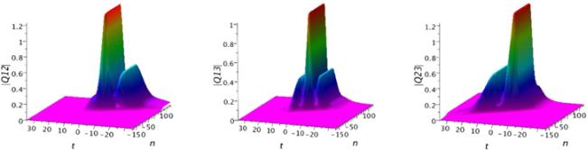
Figure 3. Two-soliton solution Qpq at y = 0 in the case of ( |
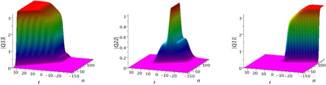
Figure 4. Two-soliton solution Qqq at y = 0 in the case of ( |
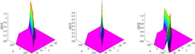
Figure 5. Two-soliton solution Qpq at y = 0 in the case of ( |
Figure 6. Two-soliton solution Qqq at y = 0 in the case of ( |
5. Remarks
If introduce a new matrix function $\tilde{Q}(n)$ by ${\chi }^{(1)}(n)={\rm{i}}\tilde{Q}(n)$ , instead of (2.5 ), then we find, from equation (2.6 ), another form of (2 + 1)-dimensional discrete three wave equation $ \begin{eqnarray}\begin{array}{c}\begin{array}{l}{{\rm{\partial }}}_{t}[{a}_{q}{\tilde{Q}}_{{pq}}(n)-{a}_{p}{\tilde{Q}}_{{pq}}(n-1)]\\ \,-\,{{\rm{\partial }}}_{y}[{b}_{q}{\tilde{Q}}_{{pq}}(n)-{b}_{p}{\tilde{Q}}_{{pq}}(n-1)]\\ \,=\,{s}_{{pq}}[{\tilde{R}}_{p}(n){\tilde{Q}}_{{pq}}(n)-{\tilde{Q}}_{{pq}}(n-1){\tilde{R}}_{q}(n)]\\ \,\,+\,{{\rm{i}}s}_{{pq}}({E}^{-}-1){\tilde{Q}}_{{pq}}(n)-{s}_{{pq}}{\tilde{Q}}_{{pr}}(n-1){\tilde{Q}}_{{rq}}(n)\\ \,\,+\,{s}_{{rq}}{\tilde{Q}}_{{pr}}(n){\tilde{Q}}_{{rq}}(n)+{s}_{{pr}}{\tilde{Q}}_{{pr}}(n-1){\tilde{Q}}_{{rq}}(n-1),\\ \,r\ne p\ne q,\end{array}\end{array}\,\end{eqnarray}$ $ \begin{eqnarray}\begin{array}{l}(1-{E}^{-})\left[{a}_{p}{\partial }_{t}{\tilde{Q}}_{{pp}}(n)-{b}_{p}{\partial }_{y}{\tilde{Q}}_{{pp}}(n)\right.\\ \quad \left.+\,\displaystyle \sum _{r\ne p}{s}_{{pr}}| {\tilde{Q}}_{{pr}}(n){| }^{2}\right]=0,\end{array}\end{eqnarray}$ where ${\tilde{R}}_{p}(n)$ have the same definition as in (2.3 ). Note that ${({\chi }^{(1)})}^{\dagger }(n)=-{\chi }^{(1)}(n)$ implies the constraint ${\tilde{Q}}^{\dagger }(n)=\tilde{Q}(n)$ , which was imposed in [25]. The N-soliton solution takes the following form $ \begin{eqnarray}\tilde{Q}=\displaystyle \frac{-1}{2\pi }{\check{Z}}^{\dagger }{\left(I+M\right)}^{-1}\check{Z},\end{eqnarray}$ where $\check{Z}$ is defined in (4.12 ).