


1. Introduction
Recently, the Event Horizon Telescope team announced the most awaiting results on the first ever image of the supermassive black hole M87* [1, 2]. This excites researchers to explore the different solutions as well as aspects of the black holes. Black hole solutions in modified theories of gravity are described to demonstrate astrophysical signatures [3] and observe the deviation from the general relativity. Since the last few decades, black hole solutions without spacetime singularities have been discussed extensively, widely known as regular black holes. A regular black hole is a singularity free solution of general relativity coupled with the nonlinear electrodynamics. Interestingly, these black holes have an event horizon but the spacetime singularity is replaced with a de Sitter core by introducing some exotic field. The initial attempt dates back to Sakharov [4] and Gliner [5] who proposed an idea to obtain a singularity free black hole solution. Fortunately, Bardeen succeeded to discover the first ever regular black hole solution [6], and after his pioneering work several regular models have been proposed so far in literature [7–13]. Although the physical source of the Bardeen black hole was described much later after his proposal in [14]. In this paper, they interpreted the physical source as a gravitational field of a nonlinear magnetic monopole of the self-gravitating magnetic field. Apart from this, Ayón–Beato–García (ABG) also obtained an exact solution of the Einstein’s field equations coupled with nonlinear electrodynamics [15], which has a self-gravitating electric charge source. The solution is a modification of the Reissner–Nordström solution and can be surrounded by the Keplerian disc. The general procedure to construct regular black hole solutions in general relativity coupled to the nonlinear electrodynamics has also been discussed [16, 17]. Many authors employed the Newman–Janis algorithm successively on regular solutions to obtain the rotating counterparts of them [18–23]. Besides, some interesting studies on the regular black hole has been explored, for instance, circular geodesic around a black hole [24–26], quasinormal modes [27], black hole shadow [28, 29], electromagnetic perturbations [30–32], gravitational lensing [33, 34], particle motion [35], and particle acceleration [36–38].
The main goal of the paper is to explore the orbital motion of the test particle by employing the phase-plane analysis on regular black holes. The phase-plane analysis is a standard approach to describe the relativistic orbits around the black hole. Previously, this analysis has been successively applied on Schwarzschild [39] to describe its relativistic orbits. The relativistic orbits of stingy black holes [40] and regular Hayward black holes [41] have also been discussed by following the same phase-plane analysis. Inspired with the previous works on this topic so far, we are going to construct the relativistic orbits of the test particle in the gravitational field of Reissner–Nordström (RN) type regular black hole. It is an exact solution of Einstein field equations coupled to the nonlinear electrodynamics, which in the asymptotic limit tends to the Reissner–Nordström [13]. The spacetime contains nonlinear electric charge due to nonlinear electrodynamics. We wish to observe the effect of charge on the relativistic orbits of the test particle as well as compare our results with relativistic orbits of the ABG black hole.
The paper is organized as follows. In section 2 , we discuss general relativistic orbits of the test particle in the gravitational field of RN-type regular black hole spacetime. The stability and phase-plane analysis investigation is the subject of section 3 . We examine the same analysis for the ABG black hole in section 4 . At the end we conclude the key results in section 5 .
2. General relativistic orbits
We start with Reissner–Nordström (RN)-type regular black hole spacetimes, which is an exact solution of general relativity coupled to the nonlinear electrodynamics. The dynamics governed by the action [13] can be written as follows $ \begin{eqnarray}{ \mathcal S }=\displaystyle \frac{1}{16\pi }\int {{\rm{d}}}^{4}x\sqrt{-g}\left(R-4L(F\right)),\end{eqnarray}$ where R is the Ricci scalar and the Lagrangian density L(F) is a nonlinear function of electromagnetic scalar $F=(1/4){F}_{\mu \nu }{F}^{\mu \nu }$ with ${F}_{\mu \nu }={{\rm{\nabla }}}_{[\mu }{A}_{\nu ]}$ . In weak field approximation, $L(F)\to F$ , which describes the Maxwell theory in weak field. The corresponding spherically symmetric spacetime metric in geometrized units (G = c = 1) is given by $ \begin{eqnarray}{{\rm{d}}{s}}^{2}=-f(r){{\rm{d}}{t}}^{2}+\displaystyle \frac{1}{f(r)}{{\rm{d}}{r}}^{2}+{r}^{2}({\rm{d}}{\theta }^{2}+{\sin }^{2}\theta {\rm{d}}{\phi }^{2}),\end{eqnarray}$ where the metric function f(r) has the following explicit form [13] $ \begin{eqnarray}f(r)=1-\displaystyle \frac{2M}{r}{{\rm{e}}}^{-{q}^{2}/2{Mr}}.\end{eqnarray}$ Here the parameters M and q represent the mass and the electric charge, respectively. Interestingly, in the asymptotic limit the metric function tends to Reissner–Nordström. This can be easily checked by expressing exponential function to the first order that turns out,
$ \begin{eqnarray*}f(r)\approx 1-2M/r+{q}^{2}/{r}^{2}.\end{eqnarray*}$
As like RN, the spacetime metric (2 ) has two horizons, but it is free from spacetime singularity.
As like RN, the spacetime metric (
Now we are going to discuss the test particle motion having rest mass m0, in the gravitational field of spacetime (2 ). First of all, let us write down the Lagrangian for a test particle, $ \begin{eqnarray}\begin{array}{rcl}{ \mathcal L } & = & \displaystyle \frac{1}{2}{m}_{0}{\left(\displaystyle \frac{{\rm{d}}{s}}{{\rm{d}}\tau }\right)}^{2}\\ & = & \displaystyle \frac{1}{2}{m}_{0}\left[-f(r){\dot{t}}^{2}+\displaystyle \frac{1}{f(r)}{\dot{r}}^{2}+{r}^{2}{\dot{\theta }}^{2}+{r}^{2}{\sin }^{2}\theta {\dot{\phi }}^{2}\right],\end{array}\end{eqnarray}$ where ${\dot{x}}^{\mu }={{\rm{d}}{x}}^{\mu }/{\rm{d}}\tau ,\tau $ is proper time, and μ = 0, 1, 2, 3. We know that the Lagrangian is a constant of motion, which implies ${ \mathcal L }=-{m}_{0}/2$ . If the test particle orbits are confined in the equatorial plane (θ = π/2), then the Lagrangian (4 ) takes the following explicit form, $ \begin{eqnarray}{ \mathcal L }=-\displaystyle \frac{1}{2}{m}_{0}=\displaystyle \frac{1}{2}{m}_{0}\left[-f(r){\dot{t}}^{2}+\displaystyle \frac{1}{f(r)}{\dot{r}}^{2}+{r}^{2}{\dot{\phi }}^{2}\right].\end{eqnarray}$ It is noticeable that the Lagrangian is independent on t and φ coordinates, which turns out two constants of motion or two conserved quantities. These conserved quantities basically are energy ϵ and angular momentum l corresponding to the t and φ coordinates, respectively. We are going to employ the Euler–Lagrange equation to compute the geodesic equations of the test particle, $ \begin{eqnarray}\displaystyle \frac{{\rm{d}}}{{\rm{d}}\tau }\left(\displaystyle \frac{\partial { \mathcal L }}{\partial {\dot{x}}^{\mu }}\right)-\displaystyle \frac{\partial { \mathcal L }}{\partial {x}^{\mu }}=0.\end{eqnarray}$ On using (6 ) we obtain the geodesics equations for the t and φ coordinates as following $ \begin{eqnarray}\begin{array}{rcl}\displaystyle \frac{\partial { \mathcal L }}{\partial t} & = & 0\Rightarrow \displaystyle \frac{\partial { \mathcal L }}{\partial \dot{t}}={m}_{0}f(r)\dot{t}=\varepsilon ,\\ \displaystyle \frac{\partial { \mathcal L }}{\partial \phi } & = & 0\Rightarrow \displaystyle \frac{\partial { \mathcal L }}{\partial \dot{\phi }}={m}_{0}{r}^{2}\dot{\phi }=l,\end{array}\end{eqnarray}$ it turns out from equation (7 ) that $ \begin{eqnarray}\dot{t}=\displaystyle \frac{\varepsilon }{{m}_{0}f(r)},\quad \dot{\phi }=\displaystyle \frac{l}{{m}_{0}{r}^{2}}.\end{eqnarray}$ On substituting (8 ) into (5 ), and after doing some algebraic simplification, we obtain the radial geodesic equation, $ \begin{eqnarray}{\dot{r}}^{2}=\displaystyle \frac{{\varepsilon }^{2}}{{m}_{0}^{2}}-f(r)-\displaystyle \frac{{l}^{2}}{{m}_{0}^{2}{r}^{2}}f(r).\end{eqnarray}$ Now we define E ≡ ϵ/m0, and rewrite $\dot{r}$ such that $ \begin{eqnarray}\dot{r}=\displaystyle \frac{{\rm{d}}{r}}{{\rm{d}}\phi }\dot{\phi }=\displaystyle \frac{l}{{m}_{0}{r}^{2}}\left(\displaystyle \frac{{\rm{d}}{r}}{{\rm{d}}\phi }\right),\end{eqnarray}$ when substituting (10 ) into equation (9 ), it gives $ \begin{eqnarray}{\left(\displaystyle \frac{{\rm{d}}{r}}{{\rm{d}}\phi }\right)}^{2}=\displaystyle \frac{{m}_{0}^{2}{r}^{4}}{{l}^{2}}{E}^{2}-\displaystyle \frac{{m}_{0}^{2}{r}^{4}}{{l}^{2}}f(r)-{r}^{2}f(r).\end{eqnarray}$ Furthermore, we introduce a new variable such that $u={r}_{+}/r$ , where ${r}_{+}$ is the event horizon of the regular black hole. Now we rewrite down the metric function (20 ), in terms of new variable u, it takes the following form $ \begin{eqnarray}\begin{array}{rcl}f(r) & = & 1-\displaystyle \frac{2{Mu}}{{r}_{+}}{{\rm{e}}}^{-{q}^{2}u/2{{Mr}}_{+}}=1-g(u),\end{array}\end{eqnarray}$ where we define function g(u) as follows $ \begin{eqnarray}g(u)=\displaystyle \frac{2{Mu}}{{r}_{+}}{{\rm{e}}}^{-{q}^{2}u/2{{Mr}}_{+}}.\end{eqnarray}$ In terms of u, we substitute ${\rm{d}}{r}=-({r}_{+}/{u}^{2}){\rm{d}}{u}$ , into the equation (11 ), which reforms $ \begin{eqnarray}{\left(\displaystyle \frac{{\rm{d}}{u}}{{\rm{d}}\phi }\right)}^{2}=2\beta ({E}^{2}-1)+2\beta g(u)-{u}^{2}+{u}^{2}g(u),\end{eqnarray}$ where the parameter β is define by $ \begin{eqnarray}\beta =\displaystyle \frac{1}{2}{\left(\displaystyle \frac{{m}_{0}{r}_{+}}{l}\right)}^{2}.\end{eqnarray}$ It is noticeable that the dimensionless parameter β has a dependency on the angular momentum as well as rest mass of the test particle. Eventually, we are in a position to discuss the general relativistic orbits for the chosen regular black hole.
3. Stability and phase-plane analysis of test particle orbits
Now we start by discussing the stability of relativistic orbits of the test particle and construct the phase-plane diagrams to understand the pattern of them. To reach that goal we introduce two new variables, x = u and y = du/dφ, such that the equation (14 ) rewritten as follows $ \begin{eqnarray}{y}^{2}=2\beta ({E}^{2}-1)+2\beta g(x)-{x}^{2}+{x}^{2}g(x).\end{eqnarray}$
Let us compute the expression of effective potential by substituting y = 0 in (16 ), thus it turns out that $ \begin{eqnarray}\begin{array}{rcl}{V}_{{\rm{eff}}}^{2}-1 & = & \displaystyle \frac{{x}^{2}}{2\beta }\left(1-\displaystyle \frac{2{Mx}}{{r}_{+}}{{\rm{e}}}^{-{q}^{2}x/2{{Mr}}_{+}}\right)\\ & & -\displaystyle \frac{2{Mx}}{{r}_{+}}{{\rm{e}}}^{-{q}^{2}x/2{{Mr}}_{+}}.\end{array}\end{eqnarray}$ Clearly, the effective potential has dependency on the charge q and the parameter β, the effect of these parameters can be examined by plotting it against x. The typical behavior of the effective potential can be seen from figure 1. For the large value of β, the curves lie below the x-axis and there is no extreme point in this case so they can directly fall into the black hole. We get extreme points of effective potential at β = 0.113 2 for q = 0.6 (see figure 1). The curve containing the extreme value is known as critical curve at which the stable circular orbits can observe (see figure 1). We now wish to check the stability of the test particle orbits in a regular black hole. To reach the goal we differentiate the effective potential (17 ) with respect to x, which gives $ \begin{eqnarray}\begin{array}{rcl}\displaystyle \frac{{{\rm{d}}{V}}_{{\rm{eff}}}^{2}}{{\rm{d}}{x}} & = & \displaystyle \frac{x}{\beta }-\displaystyle \frac{{{\rm{e}}}^{-{q}^{2}x/2{{Mr}}_{+}}}{2\beta {r}_{+}^{2}}\\ & & \times \left[{{xq}}^{2}({x}^{2}+2\beta )-2{{Mr}}_{+}(3{x}^{2}+2\beta )\right].\end{array}\end{eqnarray}$ The location of the stable and unstable orbits can be determined by solving the condition, ${{\rm{d}}{V}}_{{\rm{eff}}}^{2}/{\rm{d}}{x}=0$ for x. The stable orbits can be observed for the smallest value of x while the unstable orbits can be observed when x is largest. However, the stability of the test particle orbits can be determined by the condition ${{\rm{d}}}^{2}{V}_{{\rm{eff}}}^{2}/{{\rm{d}}{x}}^{2}\geqslant 0$ , where ${{\rm{d}}}^{2}{V}_{{\rm{eff}}}^{2}/{{\rm{d}}{x}}^{2}$ is further differentiation of equation (18 ) with respect to x, which has the following form $ \begin{eqnarray}\begin{array}{rcl}\displaystyle \frac{{{\rm{d}}}^{2}{V}_{{\rm{eff}}}^{2}}{{{\rm{d}}{x}}^{2}} & = & \displaystyle \frac{1}{\beta }-\displaystyle \frac{{{\rm{e}}}^{-{q}^{2}x/2{{Mr}}_{+}}}{4M\beta {r}_{+}^{3}}\left[{{xq}}^{4}({x}^{2}+2\beta )\right.\\ & & \left.+24{{xM}}^{2}{r}_{+}^{2}-4{{Mq}}^{2}{r}_{+}(3{x}^{2}+2\beta )\right].\end{array}\end{eqnarray}$ It should be noted that the test particle has stable circular orbit when both ${{\rm{d}}{V}}_{{\rm{eff}}}^{2}/{\rm{d}}{x}=0$ and ${{\rm{d}}}^{2}{V}_{{\rm{eff}}}^{2}/{{\rm{d}}{x}}^{2}\geqslant 0$ , conditions are satisfied together.
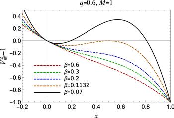
Figure 1. Plot showing the behavior of the effective potential of the test particle for RN type regular black hole β = 0.6, 0.3, 0.2, 0.113 2, 0.07. |
Now we are going to portray the phase-plane diagram by using equation (16 ) to observe the patterns of the test particle orbits around the black hole. Since the equations of motion are integrable because of the constants of motion, therefore we can construct an exact phase-plane for the RN-type black hole. We plot the graphs of phase-plane in figure 2, for different values of charge q and parameter β. It shows five different orbital trajectories corresponding to the different values of energy E2, which can be seen from figure 2. These orbital trajectories correspond to the particular value of effective potential (cf figure 2). We obtain elliptical orbits (red curve) when ${V}_{{\rm{eff}}}^{2}-1\lt 0$ , parabolic orbits (green curve) when ${V}_{{\rm{eff}}}^{2}-1=0$ , hyperbolic orbits (blue curve) when ${V}_{{\rm{eff}}}^{2}-1\gt 0$ , and separatrix (orange curve). These orbits can be easily understand by looking on the corresponding diagram of effective potential (see figure 2). We vary the charge q to obtain the corresponding phase-plane diagrams, which are portrayed in figure 3. It tell us that for each value of charge q there is a separatix that can be visualized by orange dashed lines.
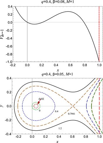
Figure 2. Plot showing the behavior of effective potential and exact phase-plane diagram of the test particle in an RN-type regular black hole ( |
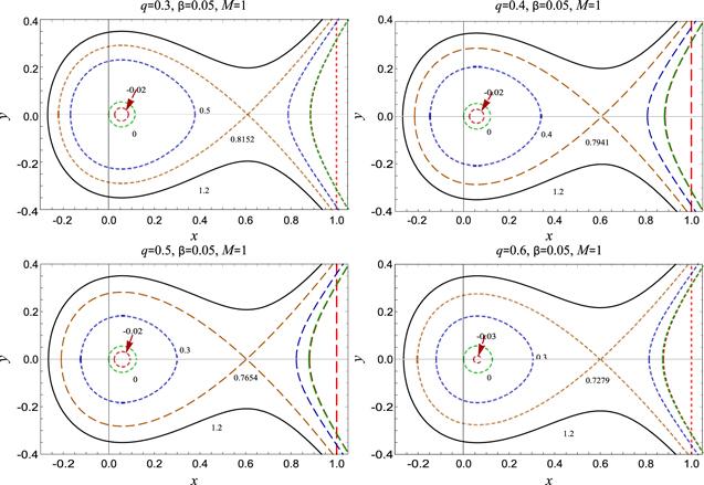
Figure 3. Plot showing various cases of the exact phase-plane diagrams for an RN-type regular black hole by varying the values of |
However, the significance of the different cases of β can be understood by the location of the separatrix in the phase-plane diagram (see the orange dashed curve in figures 2 and 3). A separatrix corresponds to the boundary that exists before the unstable orbits formation. Consequently, it represents the critical relationship between energy and angular momentum at the radii of unstable orbits. Although the numerical values of the innermost stable circular orbit’s radii rmin and energy E2 that requires us to place the test particle in these orbits are mentioned in table 1. We compute these values for suitable choices of charge q, event horizon ${r}_{+}$ , and angular momentum parameter β. We find that when the magnitude of charge q increases consequently the radius of the innermost stable circular orbit decreases. In the next section, we are going to extend our study for the ABG black hole.
Table 1. Numerical results on the innermost stable circular orbit radii (rmin) and corresponding energy for the RN-type regular black hole. |
| q | β | | E2 | rmin |
|---|---|---|---|---|
| 0.1 | 0.12 | 1.994 9 | 1.019 7 | 5.986 4 |
| 0.2 | 0.10 | 1.979 9 | 1.124 5 | 5.947 7 |
| 0.3 | 0.09 | 1.954 5 | 1.191 0 | 5.884 1 |
| 0.4 | 0.08 | 1.918 3 | 1.271 9 | 5.796 8 |
| 0.5 | 0.07 | 1.870 7 | 1.373 1 | 5.685 9 |
| 0.6 | 0.05 | 1.810 7 | 1.728 1 | 5.563 9 |
4. Ayón–Beato–García black hole
In this section, we shall discuss the phase-plane diagrams for the Ayón–Beato–García (ABG) spacetime metric [15]. As we already mentioned in the introduction that the ABG spacetime is also an exact solution of general relativity coupled to the nonlinear electrodynamics. The metric function f(r) for this spacetime has the following sort of form [15], $ \begin{eqnarray}f(r)=1-\displaystyle \frac{2{{Mr}}^{2}}{{\left({r}^{2}+{q}^{2}\right)}^{3/2}}+\displaystyle \frac{{q}^{2}{r}^{2}}{{\left({r}^{2}+{q}^{2}\right)}^{2}}.\end{eqnarray}$ It is noticeable that the metric function is more complicated in comparison to the RN-type regular black hole because of fractional power in the denominator. Even this spacetime has two distinct horizons as like the RN-type regular black hole. Now let us calculate the effective potential for the ABG black hole, which is written as follows $ \begin{eqnarray}\begin{array}{rcl}{V}_{{\rm{eff}}}^{2}-1 & = & \displaystyle \frac{{x}^{2}}{2\beta }\left(1-\displaystyle \frac{2{{Mxr}}_{+}^{2}}{{\left({r}_{+}^{2}+{q}^{2}{x}^{2}\right)}^{3/2}}+\displaystyle \frac{{q}^{2}{x}^{2}{r}_{+}^{2}}{{\left({r}_{+}^{2}+{q}^{2}{x}^{2}\right)}^{2}}\right)\\ & & -\displaystyle \frac{2{{Mxr}}_{+}^{2}}{{\left({r}_{+}^{2}+{q}^{2}{x}^{2}\right)}^{3/2}}+\displaystyle \frac{{q}^{2}{x}^{2}{r}_{+}^{2}}{{\left({r}_{+}^{2}+{q}^{2}{x}^{2}\right)}^{2}}.\end{array}\end{eqnarray}$
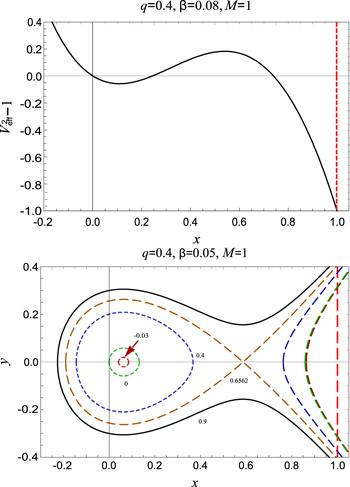
However, the first derivative of effective potential (21 ) with respect to x is given by $ \begin{eqnarray}\begin{array}{rcl}\displaystyle \frac{{{\rm{d}}{V}}_{{\rm{eff}}}^{2}}{{\rm{d}}{x}} & = & \displaystyle \frac{1}{\beta {\left({r}_{+}^{2}+{q}^{2}{x}^{2}\right)}^{3}}\left[x\{{r}_{+}^{6}+{q}^{2}{r}_{+}^{4}(5{x}^{2}+2\beta )\right.\\ & & +{q}^{4}{x}^{2}{r}_{+}^{2}(3{x}^{2}-2\beta )+{q}^{6}{x}^{6}\}\\ & & \left.-{{Mr}}_{+}^{2}\sqrt{{r}_{+}^{2}+{q}^{2}{x}^{2}}\left({r}_{+}^{2}(3{x}^{2}+2\beta )-4\beta {q}^{2}{x}^{2}\right)\right],\end{array}\end{eqnarray}$ and the second derivative with respect to x has the form, $ \begin{eqnarray}\begin{array}{l}\displaystyle \frac{{{\rm{d}}}^{2}{V}_{{\rm{eff}}}^{2}}{{{\rm{d}}{x}}^{2}}=\displaystyle \frac{1}{\beta {\left({r}_{+}^{2}+{q}^{2}{x}^{2}\right)}^{4}}\left[{r}_{+}^{8}+2{q}^{2}{r}_{+}^{6}(5{x}^{2}+\beta )\right.\\ -16\beta {q}^{4}{x}^{2}{r}_{+}^{4}-3{{Mxr}}_{+}^{2}\sqrt{{r}_{+}^{2}+{q}^{2}{x}^{2}}\{2{r}_{+}^{4}\\ \quad -\,3{q}^{2}{r}_{+}^{2}({x}^{2}+2\beta )+4\beta {q}^{4}{x}^{2}\}\\ \left.+\,2{q}^{6}{x}^{4}{r}_{+}^{2}(2{x}^{2}+3\beta )+{q}^{8}{x}^{8}\right].\end{array}\end{eqnarray}$ The phase-plane diagram for the ABG black hole and its behavior is described in figure 4. We obtain all the possible orbits, e.g., elliptical orbits (red curve) when ${V}_{{\rm{eff}}}^{2}-1\lt 0$ , parabolic orbits (green curve) when ${V}_{{\rm{eff}}}^{2}-1=0$ , hyperbolic orbits (blue curve) when ${V}_{{\rm{eff}}}^{2}-1\gt 0$ , and the separatrix (orange curve). To make the results more clear we compute the numerical values of innermost stable circular orbit's radii rmin and energy E2 that requires us to place the test particle in particular orbits (see table 2). For a comparison we look carefully on the numerical results for both of the black holes. We realize a significant difference not only in radii rmin values but also in energy E2 for fixed values of parameters q and β. The radii of event horizon have higher magnitude in case of the RN-type regular black hole in comparison to the ABG black hole. Consequently, the numerical values of radii rmin and corresponding energy E2 also have higher values in the RN-type black hole in comparison to the ABG black hole. On the other hand, the orbital motion can be used to describe the gravitational lensing for the particular black hole spacetime.
Figure 4. Plot showing the behavior of effective potential and exact phase-plane diagram of the test particle in the background of the ABG black hole ( |
Table 2. Numerical results on the innermost stable circular orbit radii (rmin) and corresponding energy for the ABG black hole. |
| q | β | | E2 | rmin |
|---|---|---|---|---|
| 0.1 | 0.12 | 1.987 4 | 1.016 8 | 5.972 4 |
| 0.2 | 0.10 | 1.948 7 | 1.109 5 | 5.893 9 |
| 0.3 | 0.09 | 1.880 4 | 1.151 1 | 5.760 4 |
| 0.4 | 0.08 | 1.775 1 | 1.183 3 | 5.564 9 |
| 0.5 | 0.07 | 1.614 2 | 1.186 5 | 5.286 3 |
| 0.6 | 0.05 | 1.324 4 | 1.212 1 | 4.901 5 |
4.1.Photon as a test particle:
If we consider the massless particle (photon), then the separatrix will be physically very important. Essentially, in this scenario the separatrix turns out to be the unstable spherical photon orbits that provides valuable information regarding the structure of the black hole. These unstable spherical photon orbits are very interesting from the astrophysical as well as the theoretical points of view. They play a crucial role in case of axially symmetric spacetimes as the shadow of the black hole could be determined with them. Basically, the black hole shadow is an optical apparent image of the black hole when it is placed between a bright object and a distant observer. Moreover, the orbital motion of spherical photon orbit around the black hole spacetimes governs the Keplerian accretion discs. It may help us to find an influence on the behaviour of the Keplerian accretion discs.
5. Concluding remarks
The regular black holes have attracted much attention from the researchers while discussing the modified theories of gravity. So far various aspects of these regular black holes have been considered in literature to understand the physical nature of them. Essentially, the growing interest motivates us to do a comprehensive study to investigate the relativistic orbital dynamics of the test particle in the gravitational field of regular black holes. We have chosen RN-type regular black hole spacetime and ABG black hole spacetime for our study. Both of the spacetimes are completely determined by their mass M and the nonlinear charge q. We calculated test particle geodesics by using the Euler–Lagrange method. Later on, a discussion on the effective potential has been taken place, and mathematical formulation of the stability analysis has also been explored.
We mainly emphasized the phase-plane analysis to demonstrate the orbits of the test particle in the gravitational field of the RN-type regular black hole and the ABG black hole. In order to explore the orbital dynamics, we have plotted the phase-plane diagrams for both of the regular black holes. Consequently, we have obtained a complete set of orbits around the black hole according to the variation of energy E2, which we classify as elliptical, parabolic, hyperbolic, and separatrix. It has been observed that the presence of charge q allowed us to portray different cases of phase-plane diagrams. As we mentioned earlier, the term separatrix, which is defined as a critical orbit, can be obtained for the precise value of the energy E2. The numerical results for E2 can be seen from the tables 1 and 2. When the amount of energy E2 is greater than the computed values, in this case there is no stable orbit. Besides, if it is less than the computed values then there are stable orbits. Moreover, we have discussed the effect of charge q on orbital motion of the test particle in both of the spacetimes. It is found that whenever there is an increase in charge q as a result the particle needs more energy to form stable orbits around the black holes. In addition, we have calculated the radii of the innermost stable circular orbits for different values of charge q and parameter β. Our results show that the radius of the innermost stable circular orbits decreases due to an increase in the amount of charge q. A comparison between the RN-type black hole and the ABG black hole results in the difference in radii of the innermost stable circular orbits as well as energy required to place the test particle in orbits. Physically, the separatrix is important because it provides a critical relationship between the energy and the angular momentum. Moreover, it splits the phase-plane into the physically distinct regions. In the case of the photon (massless particle), the separatrix corresponds to the unstable spherical photon orbits also known as photonspheres, which provides valuable information regarding the structure of the black hole. These spherical photon orbits are interesting from the astrophysical as well as the theoretical points of view. For instance, they play a crucial role in the case of axially symmetric spacetimes as the shadow of the black hole is determined with them. They also have an influence on the behaviour of the Keplerian disks.