


1. Introduction
We consider in this paper the following nonlinear Schrödinger equation with a Dirac delta potential:1 ) over the interval [−ϵ, ϵ], and then considering the limit $\varepsilon \to 0$.
$\begin{eqnarray}{\rm{i}}{\partial }_{t}{\rm{\Psi }}(x,t)=\left(-\displaystyle \frac{1}{2}{\partial }_{x}^{2}+\lambda \delta (x)+g| {\rm{\Psi }}(x,t){| }^{2}\right){\rm{\Psi }}(x,t),\end{eqnarray}$
where i is the imaginary unit, λ and g are constants, and δ(x) represents the Dirac delta function [1]. While the function $\Psi$(x, t) is continuous at x = 0, its derivative is not. Instead, we have the following matching relation $\begin{eqnarray}{\partial }_{x}{\rm{\Phi }}(0+\,,\,t)-{\partial }_{x}{\rm{\Phi }}(0-\,,\,t)=2\lambda {\rm{\Phi }}(0,t),\end{eqnarray}$
which can be obtained by firstly integrating equation (Equation (1 ) provides an idealized model for short-range interactions [2–6]. Due to the jump condition (2 ), special techniques shall be employed to discretize equation (1 ) properly. There are some useful numerical methods for solving equation (1 ). For instance, a finite element method is developed in [7], where the Dirac delta function is incorporated directly into the discretization of the problem by using the inherent integration of the method. In [8], the evolution operator of equation (1 ) is approximated by means of the Lie evolution operator. Then spectral splitting methods are implemented. Viewing the problem as an interface at the point x = 0, a so-called explicit jump immersed interface method is proposed in [9]. A weak multi-symplectic reformulation is proposed in [10, 11] for equation (1 ), enabling one to get some preserving properties. One can also regularize the Dirac delta function in equation (1 ) by using a nonsingular function [12], resulting in an equation that can be handled by some common schemes. For instance, replacing the Dirac delta function by a so-called discrete delta function [13], a wavelet collocation method is constructed in [14].
In this paper, we provide a novel method to solve equation (1 ) numerically. Rather than discretizing equation (1 ) directly, we first show in section 2 that equation (1 ) can be transformed into an equation with discontinuous drift, in which case both the solution and flux are continuous. Then we can employ the method proposed in [15] to solve the transformed equation. For the purpose of efficiency, we provide in section 3 a new finite difference scheme following the derivation procedure in [15]. Numerical experiments are conducted in section 4 to validate the proposed method. Finally, we draw conclusions in section 5 .
2. Transformation
Consider the following one-dimensional equation:3 ). It is noted that6 ) that4 ) and (7 ) that5 ) into equation (3 ) results in
$\begin{eqnarray}a{\partial }_{t}\psi (x,t)=\left[b{\partial }_{x}^{2}+V(x)+g| \psi {| }^{2}\right]\psi (x,t),\end{eqnarray}$
where $\begin{eqnarray}V(x)=\lambda \delta (x)+{V}_{0}(x)\end{eqnarray}$
with V0(x) representing a regular potential. Here a, b, g and λ are constants. Let $\begin{eqnarray}\psi (x,t)={{\rm{e}}}^{c| x| }\phi (x,t),\end{eqnarray}$
where c is a constant that will be determined later to cancel the δ function in equation ( $\begin{eqnarray}{\partial }_{x}\psi ={{\rm{e}}}^{c| x| }[c\mathrm{sgn}(x)\phi +{\partial }_{x}\phi ],\end{eqnarray}$
where the ‘$\mathrm{sgn}$’ stands for the sign function. Furthermore, using the relation ${\partial }_{x}\mathrm{sgn}(x)=2\delta (x)$, we obtain immediately from equation ( $\begin{eqnarray}{\partial }_{x}^{2}\psi ={{\rm{e}}}^{c| x| }\{{c}^{2}\phi -2c\delta (x)\phi +2c{\partial }_{x}[\mathrm{sgn}(x)\phi ]+{\partial }_{x}^{2}\phi \}.\end{eqnarray}$
Thus, it follows from equations ( $\begin{eqnarray}\begin{array}{l}\left[b{\partial }_{x}^{2}+V(x)\right]\psi ={e}^{c| x| }\{[{{bc}}^{2}+{V}_{0}(x)]\phi \\ \quad +\,(\lambda -2{bc})\delta (x)\phi +2{bc}{\partial }_{x}[\mathrm{sgn}(x)\phi ]+b{\partial }_{x}^{2}\phi \}.\end{array}\end{eqnarray}$
Therefore, the choice $c=\lambda /(2b)$ cancels the term with the δ function. In this case, we know that the substitution of the transform ( $\begin{eqnarray}\begin{array}{rcl}a{\partial }_{t}\phi & = & [{{bc}}^{2}+{V}_{0}(x)+{{g}{\rm{e}}}^{2c| x| }| \phi {| }^{2}]\phi \\ & & +\lambda {\partial }_{x}[\mathrm{sgn}(x)\phi ]+b{\partial }_{x}^{2}\phi .\end{array}\end{eqnarray}$
To solve equation (9 ) involving the sign function, two matching conditions should be imposed at x = 0, i.e. the continuity of φ and the continuity of the flux, defined by9 ) is very similar to the Fokker–Planck equation considered in [15], except the additional source term $[{{bc}}^{2}+{V}_{0}(x)+{{g}{\rm{e}}}^{2c| x| }| \phi {| }^{2}]\phi $. Therefore, it is no doubt that the numerical scheme developed in [15] can be applied directly here. However, the numerical scheme is only of second order for the case with drift-admitting jumps although it is designed to be fifth-order for the case with smooth drifts. In order to save some computational resource, we prefer to solve equation (9 ) by developing in the next section a new scheme of third order for the case with smooth drifts rather than fifth order.
$\begin{eqnarray}f(x,t)=\lambda \mathrm{sgn}(x)\phi +b{\partial }_{x}\phi .\end{eqnarray}$
In addition, it is observed that equation (3. Numerical scheme
Following the procedure in [15], we develop here a new scheme for solving equation (9 ). Using the method of line, we first consider how to discretize properly the derivative of the flux, i.e. ${\partial }_{x}f$ (see equation (10 )). The key is to use a so-called staggered grid.
Suppose that the computational domain is truncated to be [xL, xR] with xL < 0 < xR. Then we divide the domain into two subdomains, denoted by Ω1 = [xL, 0] and Ω2 = [0, xR], respectively. In each subdomain Ωi, solution points and flux points are placed uniformly, where the solution points are defined by ${x}_{1,j}={x}_{L}+(j-1/2){h}_{1}$ ($1\leqslant j\leqslant {N}_{1}$) for Ω1 and ${x}_{2,j}\,={x}_{d}+(j-1){h}_{2}$ (1 ≤ j ≤ N2) for Ω2. Here hi are the spacial steps for Ωi with ${h}_{1}=-{x}_{L}/\left({N}_{1}-1/2\right)$ and ${h}_{2}={x}_{R}/({N}_{2}\,-1/2)$, where Ni are the numbers of solution points. It is noted that ${x}_{1,{N}_{1}}={x}_{\mathrm{2,1}}=0$, meaning that x = 0 is set to be a solution point. We will see later that this setup is very important for ensuring the continuity of the solution at x = 0. In addition, we define the flux points by ${x}_{1,j+1/2}={x}_{L}+{{jh}}_{1}$ ($0\leqslant j\leqslant {N}_{1}-1$) for Ω1 and ${x}_{2,j+1/2}=(j-1/2){h}_{2}$ (1 ≤ j ≤ N2) for Ω2, such that the flux points and the solution points are staggered with each other (see also figure 1 in [15]). Then it follows immediately that both the two boundary points are flux points since ${x}_{\mathrm{1,1}/2}={x}_{L}$ and ${x}_{2,{N}_{2}+1/2}={x}_{R}$.
3.1. Spacial discretization
For the introduced staggered grid, we first evaluate the flux at flux points, and then compute the flux derivative at solution points.
3.1.1. Evaluation of the flux
Here we only present the scheme for the subdomain Ω1, while the scheme for the subdomain Ω2 can be obtained immediately by using a mirror-symmetric property of the grid points. Additionally, let us assume b > 0 in equation (9 ) without loss of generality.
At a certain time level, suppose that the values of φ are known at solution points ${x}_{1,j}$, denoted by ${\phi }_{1,j}$. Then we derive a third-order interpolation scheme to obtain the values at flux points. For stability reason, we approximate the term $\lambda \mathrm{sgn}(x)\phi $ appearing in the flux at flux points ${x}_{1,j+1/2}$ by
$\begin{eqnarray}\max \{\lambda ,0\}{\phi }_{1,j+1/2}^{-}+\min \{\lambda ,0\}{\phi }_{1,j+1/2}^{+},\end{eqnarray}$
where ${\phi }_{1,j+1/2}^{-}$ represents interpolation values by using left-biased stencils while ${\phi }_{1,j+1/2}^{+}$ are obtained by using right-biased stencils. The interpolation scheme can be described as follows. Let ${{\rm{\Phi }}}_{1}^{\pm }={[{\phi }_{1,1/2}^{\pm },{\phi }_{1,3/2}^{\pm },...,{\phi }_{1,{N}_{1}-1/2}^{\pm }]}^{{\rm{T}}}$ and ${{\rm{\Phi }}}_{1}\,={\left[{\phi }_{\mathrm{1,1}},{\phi }_{\mathrm{1,2}},...,{\phi }_{1,{N}_{1}}\right]}^{{\rm{T}}}$. Then the right-biased scheme can be expressed as ${{\rm{\Phi }}}_{1}^{+}={I}_{1}^{+}{{\rm{\Phi }}}_{1}$, where the N1 × N1 interpolation matrix ${I}_{1}^{+}$ reads $\begin{eqnarray}{I}_{1}^{+}=\left(\begin{array}{ccccc}\tfrac{15}{8} & -\tfrac{5}{4} & \tfrac{3}{8} & & \\ \tfrac{3}{8} & \tfrac{3}{4} & -\tfrac{1}{8} & & \\ & \ddots & \ddots & \ddots & \\ & & \tfrac{3}{8} & \tfrac{3}{4} & -\tfrac{1}{8}\\ & & -\tfrac{1}{8} & \tfrac{3}{4} & \tfrac{3}{8}\end{array}\right).\end{eqnarray}$
For the left-biased values, the scheme reads ${{\rm{\Phi }}}_{1}^{-}\,={I}_{1}^{-}{[{\phi }_{1,1/2}^{+},{{\rm{\Phi }}}_{1}^{{\rm{T}}}]}^{{\rm{T}}}$, where the ${N}_{1}\times ({N}_{1}+1)$ interpolation matrix is $\begin{eqnarray}{I}_{1}^{-}=\left(\begin{array}{ccccccc}1 & & & & & & \\ -\tfrac{1}{3} & 1 & \tfrac{1}{3} & & & & \\ & -\tfrac{1}{8} & \tfrac{3}{4} & \tfrac{3}{8} & & & \\ & & \ddots & \ddots & \ddots & & \\ & & & -\tfrac{1}{8} & \tfrac{3}{4} & \tfrac{3}{8} & \\ & & & & -\tfrac{1}{8} & \tfrac{3}{4} & \tfrac{3}{8}\end{array}\right).\end{eqnarray}$
Let ${{\rm{\Phi }}}_{1,x}={\left[{\left({\partial }_{x}\phi \right)}_{\mathrm{1,1}/2},{\left({\partial }_{x}\phi \right)}_{\mathrm{1,3}/2},...,{\left({\partial }_{x}\phi \right)}_{1,{N}_{1}-1/2}\right]}^{{\rm{T}}}$. Then we can get the difference scheme ${{\rm{\Phi }}}_{1,x}={A}_{1}{{\rm{\Phi }}}_{1}/{h}_{1}$, where the N1 × N1 difference matrix A1 is expressed as follows:
$\begin{eqnarray}{A}_{1}=\left(\begin{array}{cccccc}-2 & 3 & -1 & & & \\ -1 & 1 & & & & \\ \tfrac{1}{24} & -\tfrac{9}{8} & \tfrac{9}{8} & -\tfrac{1}{24} & & \\ & \ddots & \ddots & \ddots & \ddots & \\ & & \tfrac{1}{24} & -\tfrac{9}{8} & \tfrac{9}{8} & -\tfrac{1}{24}\\ & & & & -1 & 1\end{array}\right).\end{eqnarray}$
Finally, we obtain the approximation to the flux as $\begin{eqnarray}\begin{array}{rcl}{f}_{1,j+1/2} & = & \max \{\lambda ,0\}{\phi }_{1,j+1/2}^{-}+\min \{\lambda ,0\}{\phi }_{1,j+1/2}^{+}\\ & & +b{\left({\partial }_{x}\phi \right)}_{1,j+1/2}.\end{array}\end{eqnarray}$
As mentioned before, the flux ${f}_{2,j+1/2}$ for the subdomain Ω2 can be obtained by using the symmetry property of the grid. Moreover, we usually apply boundary conditions ${f}_{\mathrm{1,1}/2}\,={f}_{2,{N}_{2}+1/2}=0$ in applications.3.1.2. Compute the derivative of the flux
Theoretically, the flux is continuous at x = 0. Thus, we can derive a difference scheme for the whole computational domain [xL, xR] directly. To describe the algorithm, let us introduce the flux vector ${\boldsymbol{f}}=\left[{{\boldsymbol{f}}}_{1}^{{\rm{T}}},{{\boldsymbol{f}}}_{2}^{{\rm{T}}}\right]$ with
$\begin{eqnarray}\begin{array}{rcl}{{\boldsymbol{f}}}_{1} & = & {\left[{f}_{\mathrm{1,1}/2},{f}_{\mathrm{1,3}/2},\cdot \cdot \cdot ,{f}_{1,{N}_{1}-1/2}\right]}^{{\rm{T}}},\\ {{\boldsymbol{f}}}_{2} & = & {\left[{f}_{\mathrm{2,3}/2},{f}_{\mathrm{2,5}/2},\cdot \cdot \cdot ,{f}_{2,{N}_{2}+1/2}\right]}^{{\rm{T}}},\end{array}\end{eqnarray}$
and the derivative vector ${{\boldsymbol{f}}}_{x}=\left[{{\boldsymbol{f}}}_{1,x}^{{\rm{T}}},{{\boldsymbol{f}}}_{2,x}^{{\rm{T}}}\right]$ with $\begin{eqnarray}\begin{array}{rcl}{{\boldsymbol{f}}}_{1,x} & = & {\left[{\left({\partial }_{x}f\right)}_{\mathrm{1,1}},{\left({\partial }_{x}f\right)}_{\mathrm{1,2}},\cdot \cdot \cdot ,{\left({\partial }_{x}f\right)}_{1,{N}_{1}}\right]}^{{\rm{T}}},\\ {{\boldsymbol{f}}}_{2,x} & = & {\left[{\left({\partial }_{x}f\right)}_{\mathrm{2,2}},{\left({\partial }_{x}f\right)}_{\mathrm{2,3}},\cdot \cdot \cdot ,{\left({\partial }_{x}f\right)}_{2,{N}_{2}}\right]}^{{\rm{T}}}.\end{array}\end{eqnarray}$
Then we express the difference scheme as ${{\boldsymbol{f}}}_{x}=A{\boldsymbol{f}}$, where the entries ${a}_{j,k}$ of the difference matrix A can be obtain by using the following stencils: $\begin{eqnarray}{\left[{{\boldsymbol{f}}}_{x}\right]}_{j}=\left\{\begin{array}{ll}{{\rm{\Sigma }}}_{k=1}^{3}{a}_{j,k}{[{\boldsymbol{f}}]}_{k}, & j=1,\\ {{\rm{\Sigma }}}_{k=1}^{4}{a}_{j,k}{[{\boldsymbol{f}}]}_{j+k-2}, & 2\leqslant j\leqslant {N}_{x}-1,\\ {{\rm{\Sigma }}}_{k=1}^{3}{a}_{j,k}{[{\boldsymbol{f}}]}_{{N}_{x}+k-2}, & j={N}_{x}.\end{array}\right.\end{eqnarray}$
Here [f]k denotes the kth entry of the vector f, and ${N}_{x}={N}_{1}+{N}_{2}-1$.By using the method of Lagrangian interpolation, it is straightforward to determine the entries of A. While the stencils locate in a single domain, we have
$\begin{eqnarray}\begin{array}{rcl}\,{\left[{a}_{j,k}\right]}_{1\leqslant k\leqslant 3} & = & \left\{\begin{array}{ll}\tfrac{1}{{h}_{1}}[-1,1,0], & j=1,\\ \tfrac{1}{{h}_{2}}[0,-1,1], & j={N}_{x},\end{array}\right.\\ {\left[{a}_{j,k}\right]}_{1\leqslant k\leqslant 4} & = & \left\{\begin{array}{ll}\tfrac{1}{{h}_{1}}\left[\tfrac{1}{24},-\tfrac{9}{8},\tfrac{9}{8},-\tfrac{1}{24}\right], & 2\leqslant j\leqslant {N}_{1}-2,\\ \tfrac{1}{{h}_{2}}\left[\tfrac{1}{24},-\tfrac{9}{8},\tfrac{9}{8},-\tfrac{1}{24}\right], & {N}_{1}+2\leqslant j\leqslant {N}_{x}-1.\end{array}\right.\end{array}\end{eqnarray}$
While the stencils across the interface point x = 0, i.e. ${N}_{1}-1\leqslant j\leqslant {N}_{1}+1$, the entries can be determined as ${a}_{j,k}={d}_{j-{N}_{1}+2,k}({h}_{1},{h}_{2})$, where the expressions for ${d}_{j,k}(x,y)$ are presented in table 1.Table 1. Coefficients that determine the difference scheme ( |
| s = 1 | s = 2 | s = 3 | |
|---|---|---|---|
| ${d}_{s,1}(x,y)$ | $\tfrac{1}{20x+4y}$ | $\tfrac{4{xy}-3{y}^{2}}{3x(x+y)(3x+y)}$ | $\tfrac{2{y}^{2}}{(x+y)(x+3y)(x+5y)}$ |
| ${d}_{s,2}(x,y)$ | $-\tfrac{7x+2y}{6{x}^{2}+2{xy}}$ | $\tfrac{-12{xy}+3{y}^{2}}{x(x+y)(x+3y)}$ | $-\tfrac{4x+5y}{4{xy}+4{y}^{2}}$ |
| ${d}_{s,3}(x,y)$ | $\tfrac{5x+4y}{4{x}^{2}+4{xy}}$ | $-\tfrac{3{x}^{2}-12{xy}}{y(x+y)(3x+y)}$ | $\tfrac{2x+7y}{2{xy}+6{y}^{2}}$ |
| ${d}_{s,4}(x,y)$ | $-\tfrac{2{x}^{2}}{(x+y)(3x+y)(5x+y)}$ | $\tfrac{3{x}^{2}-4{xy}}{3y(x+y)(x+3y)}$ | $-\tfrac{1}{4x+20y}$ |
3.2. Time-marching scheme
After discretizing the derivative of the flux, we obtain from equation (3 ) an ordinary differential system, which can be solved by a time-marching scheme. In this paper, the third-order Runge–Kutta scheme as used in [15] is employed (see equations (30 ) and (31 ) therein). If not stated otherwise, the time step is chosen to be $0.01\min \{{h}_{1}^{2},{h}_{2}^{2}\}$.
4. Numerical examples
In this section, we solve several problems numerically to show the validity of the aforementioned method. To measure the convergence rate, we introduce the L2-norm error, defined by
$\begin{eqnarray}{L}^{2}{\rm{error}}={\left[\displaystyle \sum _{j=1}^{{N}_{1}-1}{e}_{1,j}^{2}{h}_{1}+\displaystyle \frac{1}{2}{e}_{1,{N}_{1}}^{2}\left({h}_{1}+{h}_{2}\right)+\displaystyle \sum _{j=2}^{{N}_{2}}{e}_{2,j}^{2}{h}_{2}\right]}^{1/2},\end{eqnarray}$
and the ${L}^{\infty }$-norm error $\begin{eqnarray}{L}^{\infty }{\rm{error}}=\mathop{\max }\limits_{i,j}\left|{e}_{i,j}\right|,\end{eqnarray}$
where ei,j are the errors between numerical results and analytic solutions. Then the numerical convergence rate is measured by $\begin{eqnarray}{\rm{rate}}=-\mathrm{ln}\left({E}_{M}/{E}_{N}\right)/\mathrm{ln}(M/N),\end{eqnarray}$
where EM and EN are the errors corresponding to the cases with M and N solution points, respectively.4.1. Stationary nonlinear Schrödinger equation
At first, we consider the stationary nonlinear Schrödinger equation23 ) directly, we can solve the following time-dependent nonlinear Schrödinger equation23 ).
$\begin{eqnarray}\left(-\displaystyle \frac{1}{2}{\partial }_{x}^{2}+\lambda \delta (x)+g| \psi {| }^{2}\right)\psi =\mu \psi ,\end{eqnarray}$
where λ, g and μ are constants. Rather than solving equation ( $\begin{eqnarray}{{\rm{\Psi }}}_{t}=\left(\displaystyle \frac{1}{2}{\partial }_{x}^{2}-\lambda \delta (x)+\mu -g| {\rm{\Psi }}{| }^{2}\right){\rm{\Psi }}\end{eqnarray}$
until $\Psi$t reaches the machine zero. Then we obtain equivalently the solution of equation (It is obvious that equation (24 ) is in the form of the general equation considered in equation (3 ). Thus the algorithm presented in the previous sections can be applied directly. Here we just specify the initial condition for equation (24 ) to be Gaussian, i.e.
$\begin{eqnarray}{\rm{\Psi }}(x,0)=\displaystyle \frac{1}{\sqrt{2\pi {\tau }_{0}}}{{\rm{e}}}^{-{x}^{2}/\left(2{\tau }_{0}\right)}\end{eqnarray}$
with τ0 chosen to be 0.01. In the following two cases, we set the computational domains to be large enough, enabling us to impose the zero flux boundary condition $\begin{eqnarray}f\left({x}_{L},t\right)=f\left({x}_{R},t\right)=0.\end{eqnarray}$
In addition, the computation is stopped until the residue, defined by $\begin{eqnarray}{{\rm{Res}}}^{n}=\mathop{\max }\limits_{j}| {{\rm{\Psi }}}_{j}^{n}-{{\rm{\Psi }}}_{j}^{n-1}| ,\end{eqnarray}$
reaches the machine zero.4.1.1. Linear case
When g = 0, equation (23 ) degenerates to a linear equation, which admits a bound state solution [16]24 ) and obtain the numerical solution as shown in figure 1(a). The convergence process of the numerical solution is shown in figure 1(b). The test of accuracy in table 2 demonstrates that second-order accuracy is achieved, as expected.
$\begin{eqnarray}\psi (x)={{\rm{e}}}^{\lambda | x| }\end{eqnarray}$
with μ = −λ2/2. Here we choose λ = −1/2 and truncate the computational domain to be [−20, 20]. Then we solve equation (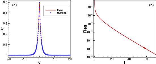
Figure 1. Numerical results for equation ( |
Table 2. Accuracy test for equation ( |
| N | L2 error | Rate | ${L}^{\infty }$ error | Rate |
|---|---|---|---|---|
| 200 | 4.05E-04 | 4.08E-04 | ||
| 400 | 1.03E-04 | 1.97 | 1.03E-04 | 1.98 |
| 800 | 2.58E-05 | 2.00 | 2.59E-05 | 1.99 |
| 1600 | 6.49E-06 | 1.99 | 6.50E-06 | 1.99 |
4.1.2. Nonlinear case
For $g\ne 0$, the nonlinear term in equation (24 ) comes into play. Here we confine the study to the case with g = 1, which admits the analytic solution [17]23 ) at x = 0; see equation (2 ). In addition, k is set as $k=-\lambda -1/2$ such that ${\int }_{-\infty }^{\infty }| \psi (x){| }^{2}{\rm{d}}{x}=1$.
$\begin{eqnarray}\psi (x)=\left\{\begin{array}{ll}-k\,\mathrm{cosech}\left(k\left(x+{x}_{0}\right)\right), & x\lt 0,\\ k\,\mathrm{cosech}\left(k\left(x-{x}_{0}\right)\right), & x\gt 0\end{array}\right.\end{eqnarray}$
if $\mu =-{(\lambda -1/2)}^{2}/2$. Here x0 is determined by the equality $\begin{eqnarray}\tanh \left({{kx}}_{0}\right)=k/\lambda ,\end{eqnarray}$
which is a consequence of the jump condition of equation (Here we set λ = −1 and truncate the computational domain to be [−15, 15]. As we can see from figure 2(a), the numerical results match well with the analytic solution. The convergence process of the numerical solution is shown in figure 2(b). The expected second-order convergence rate is also achieved as shown in table 3.
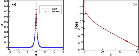
Figure 2. Numerical results for equation ( |
Table 3. Accuracy test for equation ( |
| N | L2 error | Rate | ${L}^{\infty }$ error | Rate |
|---|---|---|---|---|
| 100 | 6.27E-03 | 9.84E-03 | ||
| 200 | 1.56E-03 | 2.00 | 2.51E-03 | 1.96 |
| 400 | 3.89E-04 | 2.00 | 6.23E-04 | 2.01 |
| 800 | 9.70E-05 | 2.00 | 1.54E-04 | 2.01 |
4.2. Time-dependent nonlinear Schrödinger equation
Now we are trying to solve the time-dependent nonlinear Schödinger equation (1 ) [11]. Since $\Psi$ is a complex number for fixed x and t, we shall assume ${\rm{\Psi }}=p(x,t)+{\rm{i}}q(x,t)$ and plug it into equation (1 ) to obtain a couple of equations
$\begin{eqnarray}{{\rm{\partial }}}_{t}p=\left(-\displaystyle \frac{1}{2}{{\rm{\partial }}}_{x}^{2}+\lambda \delta (x)+g({p}^{2}+{q}^{2})\right)q,\end{eqnarray}$
$\begin{eqnarray}-{{\rm{\partial }}}_{t}q=\left(-\displaystyle \frac{1}{2}{{\rm{\partial }}}_{x}^{2}+\lambda \delta (x)+g({p}^{2}+{q}^{2})\right)p.\end{eqnarray}$
Then we can use the proposed numerical method to solve this system.When g = 1, equation (1 ) possesses the analytic solution29 ). We choose λ = −0.7 and set the initial condition as $\Psi$(x, 0) according to equation (33 ). The computational domain is truncated to be [−20, 20]. Figure 3 shows that the numerical results of the real and imaginary parts match well with the analytic solutions at time t = 1. In this case, second-order accuracy is still observed, as shown in table 4.
$\begin{eqnarray}{\rm{\Psi }}(x,t)=\psi (x)\exp \left({\rm{i}}{\left(2\lambda -1\right)}^{2}t/8\right),\end{eqnarray}$
where $\Psi$(x) is defined by equation (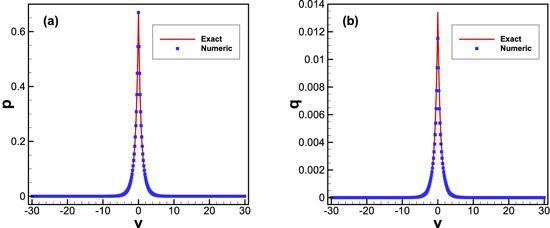
Figure 3. Numerical solution of equation ( |
Table 4. Accuracy test for equation ( |
| p | q | |||||||
|---|---|---|---|---|---|---|---|---|
| N | L2 error | Rate | ${L}^{\infty }$ error | Rate | L2 error | Rate | ${L}^{\infty }$ error | Rate |
| 200 | 5.92E-04 | 1.22E-03 | 1.55E-03 | 1.90E-03 | ||||
| 400 | 1.48E-04 | 2.00 | 3.04E-04 | 2.00 | 3.93E-04 | 1.98 | 4.88E-04 | 1.96 |
| 800 | 3.82E-05 | 1.95 | 7.49E-05 | 2.02 | 9.94E-05 | 1.98 | 1.24E-04 | 1.97 |
| 1600 | 9.80E-06 | 1.96 | 1.85E-05 | 2.02 | 2.50E-05 | 1.99 | 3.11E-05 | 1.99 |
5. Conclusions
To conclude, we have proposed in this paper a transform for the one-dimensional nonlinear Schrödinger equation with a Dirac delta potential, such that the annoying Dirac delta function can be canceled out. For the transformed equation without the delta function, we have provided an efficient second-order finite difference method. In the numerical experiments, we have considered both stationary solutions and time-dependent solutions. All the computed results validate the new method, which is second-order.