


1. Introduction
Recently, the study of soliton molecules has attracted increasing attention. Soliton molecules, called a soliton complex, were proposed by Akhmediev in 2000 [1]. Soliton molecules are a bound state consisting of multiple solitons in the optical cavity at the same time [2–5]. It has been observed experimentally in optics [2, 4, 6]. Solitons, particle-like excitations ubiquitous in many fields of physics, have been shown to exhibit bound states akin to molecules, such as plasmas physics [7], optics [8], fluid dynamics [9], and Bose–Einstein condensates [10] and complex networks [11]. The formation of such temporal soliton bound states and their internal dynamics have been observed with difficulty using direct experimental observation. And research has shown that real-time detection in resolving interactions in complex nonlinear systems is of great importance, and includes the dynamics of soliton bound states, breathers, and rogue waves.
As we all know, exact solutions for the nonlinear evolution equations (NLEEs) have been applied in the nonlinear science fields. Rational solutions of many NLEEs have been investigated by researchers [12–17]. Among these rational solutions, lump solutions, breather wave solutions, and rogue wave solutions are hot points all the time. Moreover, the mixed solution is not just specific for the (2+1)-dimensional NLEEs. For the much simpler (1+1)-dimensional NLEEs, such a solution is not unusual in the vector counterparts [18–21]. The mixed solutions consisting of lump solutions with other types of solutions attract a lot of attention, and include lump-solitons [22], lump-kink solutions [23], and resonance stripe solitons [13, 24, 25]. More similar mixed solutions have been analyzed [26–28]. For breather interaction in the NLEEs, super-regular breathers are also a hot point. A great deal of work has been carried out [29–33]. In [34], Lou gave the soliton molecules and asymmetric solitons of three (1+1)-dimensional integrable cases via velocity resonance, which are the fifth order Korteweg–de Vries (KdV) equation, the Sawada–Kotera (SK) equation and the Kaup–Kupershmidt (KK) equation. Thus, we start to think about other integrable equations and try to find the soliton molecules, asymmetric solitons, and the new types of mixed solutions, such as the mixed breather-soliton molecule solution, the mixed lump-soliton molecule solution, and the mixed solution composed of lump waves, breather waves, and soliton molecules (asymmetric solitons). In this paper, we focus on a (2 + 1)-dimensional bidirectional SK (bSK) equation [35]2 ) through the normal form of equation (1) in [41, 42]. Moreover, it is often preferable in many physical situations to have an equation which allows us to model waves that propagate in opposite directions. Therefore, the study of a bSK equation is quite interesting. Some work has been carried out on investigation of the bSK equation (1 ). For instance, Darboux and Bäklund transformations of the bSK equation (1 ) are derived, and some approximate and exact solutions of the bSK equation (1 ) are obtained by means of Maple, such as solitary wave solutions, doubly periodic solutions, and two-soliton solutions [43, 44]. However, to the best of the authors’ knowledge, soliton molecules, asymmetric solitons and the mixed solutions between breather waves (lump waves) and soliton molecules (asymmetric solitons), and the mixed solutions composed of lump waves, breather waves, and soliton molecules (asymmetric solitons) for the bSK equation (1 ) have not been investigated before.
$\begin{eqnarray}\begin{array}{l}-45{u}^{2}{u}_{x}-15{{uu}}_{{xxx}}-15{u}_{x}{u}_{{xx}}-15{{uu}}_{t}-15{u}_{x}{\left({\partial }_{x}\right)}^{-1}({u}_{t})\\ \quad +\,5{\left({\partial }_{x}\right)}^{-1}{u}_{{tt}}-5{u}_{{xxt}}-{u}_{{xxxxx}}+9{u}_{y}=0,\end{array}\end{eqnarray}$
where $\begin{eqnarray}\begin{array}{l}{\left({\partial }_{x}\right)}^{-n}={\left(\displaystyle \frac{d}{{d}_{x}}\right)}^{-n}.\end{array}\end{eqnarray}$
It was formulated there as a bidirectional generalization of the SK equation $\begin{eqnarray}\begin{array}{l}{u}_{t}+45{u}^{2}{u}_{x}-15{u}_{x}{u}_{{xx}}-15{{uu}}_{{xxx}}+{u}_{{xxxxx}}=0.\end{array}\end{eqnarray}$
The SK equation is an important unidirectional nonlinear evolution equation. Its mathematical properties are well documented in the literature [36–40]. The authors pointed out its bidirectional nature and relation to the SK equation (Motivated by the goal of making further progress with the bSK equation, we introduce a new possibility, the velocity resonant mechanism, to form soliton molecules of the (2 + 1)-dimensional bSK equation. Under the resonant mechanism, asymmetric solitons can be generated by changing the distance between two solitons of molecules. And we can obtain the mixed breather-soliton molecule solution by the module resonance of the wave number and partial velocity resonance, and the mixed lump-soliton molecule solution by partial velocity resonance and partial long wave limits. The rest of the paper is organized as follows: in section 2 , we give soliton molecules and asymmetric solitons of the bSK equation. In sections 3 and 4 , based on the N-soliton solution, the mixed breather-soliton molecule solution and the mixed lump-soliton molecule solution are yielded. In section 5 , we obtain the mixed solutions composed of a lump wave, a breather wave, and a soliton molecule (asymmetric solitons). And the general case for the mixed solution is given. Our results are summarised in the final section.
2. Soliton molecules and asymmetric solitons of the (2 + 1)-D bSK equation
In this section, we focus on soliton molecules of the (2 + 1)-dimensional bSK equation (1 ). The Hirota bilinear method in soliton theory provides a powerful approach to looking for exact solutions. Within the Hirota bilinear formulation, solitons can be usually generated as follows4 ), we introduce a novel type of resonant conditions:
$\begin{eqnarray}\begin{array}{rcl}u & = & 2{\left(\mathrm{ln}f\right)}_{{xx}},\\ f & = & \displaystyle \sum _{\mu =0,1}\exp \left(\displaystyle \sum _{i=1}^{N}{\mu }_{i}{\xi }_{i}+\displaystyle \sum _{i\lt j}^{N}{\mu }_{i}{\mu }_{j}{A}_{{ij}}\right),\end{array}\end{eqnarray}$
where $\begin{eqnarray}\begin{array}{l}u=u(x,y,t),\\ {\xi }_{i}={k}_{i}x+{p}_{i}y+{w}_{i}t+{\phi }_{i},1\lt i\lt N,\\ 9{p}_{s}{k}_{s}-{k}_{s}^{6}-5{k}_{s}^{3}{w}_{s}+5{w}_{s}^{2}=0,\end{array}\end{eqnarray}$
and $\begin{eqnarray}\begin{array}{l}\exp ({A}_{{ij}})=-\displaystyle \frac{{\left({k}_{i}-{k}_{j}\right)}^{6}+5{\left({k}_{i}-{k}_{j}\right)}^{3}({w}_{i}-{w}_{j})-9({p}_{i}-{p}_{j})({k}_{i}-{k}_{j})-5{\left({w}_{i}-{w}_{j}\right)}^{2}}{{\left({k}_{i}+{k}_{j}\right)}^{6}+5{\left({k}_{i}+{k}_{j}\right)}^{3}({w}_{i}+{w}_{j})-9({p}_{i}+{p}_{j})({k}_{i}+{k}_{j})-5{\left({w}_{i}+{w}_{j}\right)}^{2}}.\end{array}\end{eqnarray}$
To find nonsingular analytical resonant excitations from u in equation (| (1) ${k}_{i}\ne \pm {k}_{j},{p}_{i}\ne \pm {p}_{j};$ | |
| (2) the velocity resonance, $\begin{eqnarray}\displaystyle \frac{{k}_{i}}{{k}_{j}}=\displaystyle \frac{{w}_{i}}{{w}_{j}}=\displaystyle \frac{{p}_{i}}{{p}_{j}}.\end{eqnarray}$ Under the resonant conditions, we can select appropriate solution parameters, which is certain to cause solitons to form a soliton molecule or an asymmetric soliton through calculation. Next, we take N = 2 as an example to see this fact. To exhibit one soliton molecule structure, a two-soliton solution needs to satisfy the following resonance condition: the velocity resonance is $\begin{eqnarray}{k}_{2}=\sqrt{-\displaystyle \frac{{k}_{1}^{3}+5{w}_{1}}{{k}_{1}}},{w}_{2}=\displaystyle \frac{\sqrt{-\tfrac{{k}_{1}^{3}+5{w}_{1}}{{k}_{1}}}{w}_{1}}{{k}_{1}}\end{eqnarray}$ or $\begin{eqnarray}{k}_{2}=-\sqrt{-\displaystyle \frac{{k}_{1}^{3}+5{w}_{1}}{{k}_{1}}},{w}_{2}=-\displaystyle \frac{\sqrt{-\tfrac{{k}_{1}^{3}+5{w}_{1}}{{k}_{1}}}{w}_{1}}{{k}_{1}},\end{eqnarray}$ and parameter selections are as follows: $\begin{eqnarray}\begin{array}{rcl}{w}_{1} & = & \displaystyle \frac{19}{5},{k}_{1}=-\displaystyle \frac{5}{2},{k}_{2}=\displaystyle \frac{3\sqrt{3}\sqrt{5}}{10},\\ {w}_{2} & = & -\displaystyle \frac{57\sqrt{3}\sqrt{5}}{125},{\phi }_{1}=0,{\phi }_{2}=10.\end{array}\end{eqnarray}$ |
From figure 1, one can clearly understand the soliton molecule structure of the (2+1)-dimensional bSK equation, and find that there are obvious differences between two solitons in the molecule, although they possess identical velocities. Their height and width are visibly different. And it is interesting that parameter φi decides the distance. When they are close enough, the molecules look like one peak soliton, which is called an asymmetric soliton. Thus, an asymmetric one-soliton solution will be generated from the soliton molecule. We take the same parameters as those in figure 1, except for ${\phi }_{2}=\tfrac{41}{10}$. The plots of the asymmetric soliton are shown in figure 2.
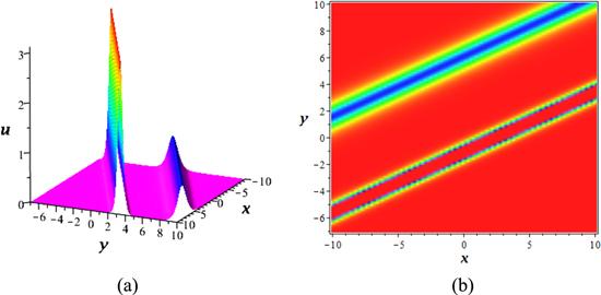
Figure 1. (a): A three-dimensional plot of the soliton molecule of the (2+1)-dimensional bSK equation; and (b) the density plots of the soliton molecule structure. |
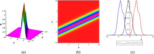
Figure 2. (a): A three-dimensional plot of the asymmetric soliton of the (2+1)-dimensional bSK equation; (b) the density plots of the asymmetric soliton; and (c) the two-dimensional plot when x = 0 at t = −5, 0, 5. |
As we all know, the interactions among solitons for the bSK equation are elastic. Therefore, we believe that the interactions among soliton molecules are also elastic. To illustrate this elastic phenomena between two soliton molecule solutions, we select suitable parameters for equation (4 ) and N = 4:
$\begin{eqnarray}\begin{array}{rcl}{k}_{1} & = & \displaystyle \frac{4}{5},{k}_{2}=\displaystyle \frac{1\sqrt{2677}\sqrt{700}}{700},{k}_{3}=-\displaystyle \frac{1}{2},{k}_{4}=-\displaystyle \frac{\sqrt{37}\sqrt{12}}{12},\\ {w}_{1} & = & -\displaystyle \frac{5}{7},{w}_{2}=-\displaystyle \frac{\sqrt{2677}\sqrt{700}}{784},{w}_{3}=\displaystyle \frac{1}{3},{w}_{4}=\displaystyle \frac{\sqrt{37}\sqrt{12}}{18},\\ {\phi }_{1} & = & -10,{\phi }_{2}=10,{\phi }_{3}=-5,{\phi }_{4}=10.\end{array}\end{eqnarray}$
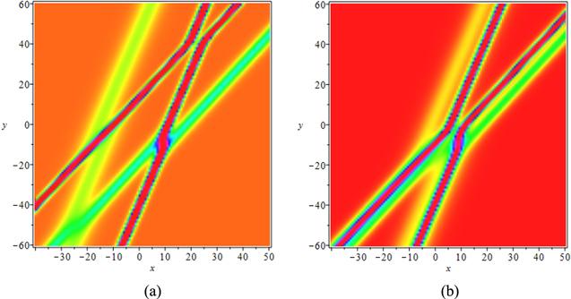
Figure 3. (a): The density plots of the elastic interaction properties for two soliton molecules of the (2+1)-dimensional bSK equation; (b) the density plots of the elastic interaction properties for two asymmetric solitons with parameters ( |
3. Mixed solutions between soliton molecules and breathers of the bSK equation
In this section, we will study the mixed solution between soliton molecules and breathers of the (2+1)-dimensional bSK equation. To obtain the mixed solution, we need the four-soliton solutions of equation (1 ), and the first two solitons must satisfy the velocity resonance; the other two solitons satisfy the module resonance of the wave numbers ${k}_{i}=\overline{{k}_{j}}$ and ${w}_{i}=\overline{{w}_{j}}$. We select the following suitable parameters in equation (4 ):
$\begin{eqnarray}\begin{array}{rcl}{k}_{1} & = & -\displaystyle \frac{5}{2},{k}_{2}=\displaystyle \frac{3\sqrt{3}\sqrt{5}}{10},{w}_{1}=\displaystyle \frac{19}{5},\\ {w}_{2} & = & -\displaystyle \frac{57\sqrt{3}\sqrt{5}}{125},{\phi }_{1}=0,{\phi }_{2}=35,\\ {k}_{3} & = & \displaystyle \frac{1}{4}-\displaystyle \frac{1}{2}{\rm{i}},{k}_{4}=\displaystyle \frac{1}{4}+\displaystyle \frac{1}{2}{\rm{i}},{w}_{3}=\displaystyle \frac{1}{3},\\ {w}_{4} & = & \displaystyle \frac{1}{3},{\phi }_{3}=0,{\phi }_{4}=0.\end{array}\end{eqnarray}$
The plots of the mixed solution between soliton molecules and breathers are shown in figure 4(a). As we can see, the interactions between soliton molecules and breathers are still elastic. We will naturally consider the mixed solution between the asymmetric soliton molecule and breathers. We know that the asymmetric soliton is generated from soliton molecules with identical parameter selections, except for φi. Thus, one can obtain the mixed solution between the asymmetric soliton molecule and breathers. Figure 4(c) displays the elastic interaction properties of the mixed solution between the asymmetric soliton molecule and breathers.
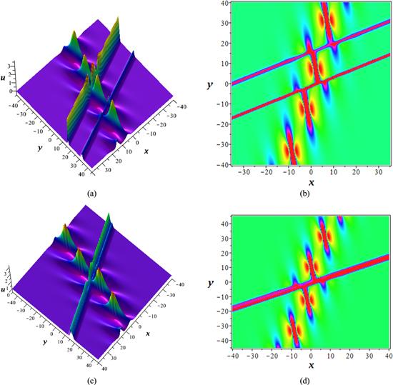
Figure 4. (a) A three-dimensional plot of a mixed solution between soliton molecules and breathers with the parameters in equation ( |
4. Mixed solutions between soliton molecules and lumps of the bSK equation
In this section, we will study a mixed solution between soliton molecules and lumps of the (2+1)-dimensional bSK equation. We can apply a partial velocity resonance and a partial long wave limit to the four-soliton solution of equation (1 ) to obtain the mixed solutions consisting of lump waves and soliton molecules or asymmetric solitons. To display the collision lump wave with soliton molecules, we take some suitable parameters for equation (4 ) as follows:1 ) by taking a long wave limit $(\epsilon \to 0)$. Therefore, we can exhibit plots of the collision lump wave with the soliton molecules in figure 5. Similarly, we consider the mixed lump-asymmetric soliton solution; the parameter selection is the same as equation (13 ), except for φ2. The plot is shown in figure 6.
$\begin{eqnarray}\begin{array}{rcl}N & = & 4,{k}_{1}=-\displaystyle \frac{5}{2},{k}_{2}=\displaystyle \frac{3\sqrt{3}\sqrt{5}}{10},{w}_{1}=\displaystyle \frac{19}{5},\\ {w}_{2} & = & -\displaystyle \frac{57\sqrt{3}\sqrt{5}}{125},{\phi }_{1}=0,{\phi }_{2}=10,\\ {k}_{3} & = & (1-{\rm{i}})\epsilon ,{k}_{4}=(1+{\rm{i}})\epsilon ,\\ {w}_{3} & = & \displaystyle \frac{7\epsilon }{2},{w}_{4}=\displaystyle \frac{7\epsilon }{2},{\phi }_{3}={\rm{i}}\pi ,{\phi }_{4}={\rm{i}}\pi .\end{array}\end{eqnarray}$
Then, we can obtain the mixed solution of equation (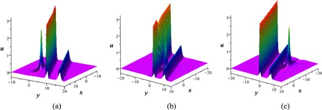
Figure 5. Time evolution of the mixed lump-soliton molecule solution of equation ( |
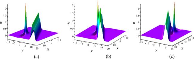
Figure 6. Time evolution of the mixed lump-asymmetric soliton solution of equation ( |
5. Mixed solutions consisting of soliton molecules, breathers, and lumps of the bSK equation
In this section, we will introduce the mixed solutions consisting of soliton molecules (asymmetric solitons), breathers, and lumps of the bSK equation. Similarly, these mixed solutions still need to satisfy the resonant condition, and take the partial long wave limit.
More generally, we can take the following parameter constraints in equation (4 ) to obtain the mixed solutions composed of m soliton molecules, n breather waves, and q lump waves.
$\begin{eqnarray}\begin{array}{rcl} & & \displaystyle \frac{{k}_{1}}{{k}_{2}}=\displaystyle \frac{{w}_{1}}{{w}_{2}}=\displaystyle \frac{{p}_{1}}{{p}_{2}},\cdot \cdot \cdot ,\,\displaystyle \frac{{k}_{2m-1}}{{k}_{2m}}=\displaystyle \frac{{w}_{2m-1}}{{w}_{2m}}=\displaystyle \frac{{p}_{2m-1}}{{p}_{2m}},\\ & & {\xi }_{2m+1}=\overline{{\xi }_{2m+2}},\cdot \cdot \cdot ,\,{\xi }_{2m+2n-1}=\overline{{\xi }_{2m+2n}},\\ & & {k}_{2m+2n+1}={K}_{2m+2n+1}\epsilon ,{k}_{2m+2n+2}=\overline{{K}_{2m+2n+1}}\epsilon ,\cdot \cdot \cdot ,\\ & & {k}_{2m+2n+2q-1}={K}_{2m+2n+2q-1}\epsilon ,\\ & & {k}_{2m+2n+2q}=\overline{{K}_{2m+2n+2q-1}}\epsilon ,\\ & & {w}_{2m+2n+1}={W}_{2m+2n+1}\epsilon ,{w}_{2m+2n+2}=\overline{{W}_{2m+2n+1}}\epsilon ,\cdot \cdot \cdot ,\\ & & {w}_{2m+2n+2q-1}={W}_{2m+2n+2q-1}\epsilon ,\\ & & {w}_{2m+2n+2q}=\overline{{W}_{2m+2n+2q-1}}\epsilon ,\\ & & {\phi }_{2m+2n+1}=\pi {\rm{i}},{\phi }_{2m+2n+2}=\pi {\rm{i}},\cdot \cdot \cdot ,\,{\phi }_{2m+2n+2q}=\pi {\rm{i}}.\end{array}\end{eqnarray}$
To clearly describe the interaction phenomenon, we take a simple example for N = 6. To obtain the mixed solution, k1, k2, w1, and w2 must satisfy the resonant condition, and k5, k6, w5, and w6 satisfy the conjuation condition. Then, we take a long wave limit on k3, k4, w3, w4 ($\epsilon \to 0$), the parameter selections as follows:
$\begin{eqnarray}\begin{array}{rcl}{k}_{1} & = & -\displaystyle \frac{5}{2},{k}_{2}=\displaystyle \frac{3\sqrt{3}\sqrt{5}}{10},{w}_{1}=\displaystyle \frac{19}{5},\\ {w}_{2} & = & -\displaystyle \frac{57\sqrt{3}\sqrt{5}}{125},{\phi }_{1}=0,{\phi }_{2}=35,\\ {k}_{3} & = & (2-{\rm{i}})\epsilon ,{k}_{4}=(2+{\rm{i}})\epsilon ,{w}_{3}=(9/2)\epsilon ,\\ {w}_{4} & = & (9/2)\epsilon ,{\phi }_{3}=\pi {\rm{i}},{\phi }_{4}=\pi {\rm{i}},\\ {k}_{5} & = & \displaystyle \frac{1}{4}-\displaystyle \frac{1}{2}{\rm{i}},{k}_{6}=\displaystyle \frac{1}{4}+\displaystyle \frac{1}{2}{\rm{i}},\\ {w}_{5} & = & \displaystyle \frac{1}{3},{w}_{6}=\displaystyle \frac{1}{3},{\phi }_{5}=0,{\phi }_{6}=0.\end{array}\end{eqnarray}$
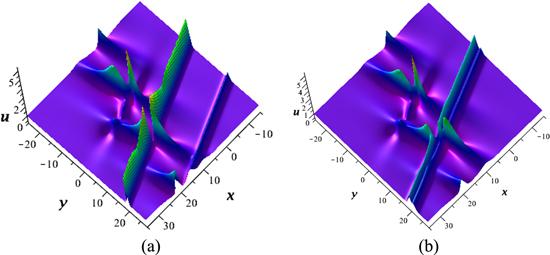
Figure 7(a) displays the mixed solutions between a soliton molecule, a lump wave, and a breather wave described by equation (4 ). We can get the mixed solution consisting of a lump wave, a breather wave, and asymmetric solitons shown in figure 7(b) by changing the distance between the two solitons in the molecule. From the plots, we can find that this interaction phenomenon is quite interesting. We obtain the mixed solutions between a soliton molecule, a lump wave, and a breather wave with parameters in equation (15 ). As time goes on, we see that the distance between the two solitons in the molecule is growing closer. At the same time, we can obtain the mixed solution between an asymmetric soliton, a lump wave, and a breather wave with the parameter selections in equation (15 ), except for φ2 = −3. In other words, the phase position φ decides the interaction phenomenon. The interaction between these waves is also elastic.
Figure 7. (a) Elastic interaction properties between a soliton molecule, a lump wave, and a breather wave for equation ( |
6. Conclusion
In this paper, we investigated soliton molecules, asymmetric solitons, and the mixed solutions between breather wave (lump wave) and soliton molecules (soliton molecules), and mixed solutions composed of soliton molecules (asymmetric solitons), lump waves, and breather waves of the (2+1)-dimensional bSK equation. And we have obtained the mixed breather-soliton molecule solution by the module resonance of the wave number and partial velocity resonance, and the mixed lump-soliton molecule solution by the partial velocity resonance and partial long wave limits. At the same time, we present three-dimensional plots and density plots of these solutions. In figure 1, it is shown that the two solitons in the molecule possess different heights and widths. Asymmetric solitons are shown in figure 2. Figure 3 indicates that the collision of two soliton molecules is elastic. The mixed solutions between soliton molecules (asymmetric soliton) and a breather wave are shown in figure 4. From figures 5 and 6, we can see the three-dimensional plots of the mixed solutions between soliton molecules (asymmetric soliton) and lump waves, respectively, at three different times. The mixed solutions consisting of soliton molecules (asymmetric solitons), lump waves, and breather waves are also obtained; see figure 7. We also give the general restrictions for obtaining these new mixed solutions containing m soliton molecules, n breather waves, and q lump waves. Finally, it is expected that these results can be useful in helping one to realize the dynamical behavior of nonlinear waves in fluid fields, and may provide some new perspectives to study the soliton molecules of nonlocal systems. Moreover, we will study super-regular breathers of the (2+1)-dimensional bSK equation in the future.