


1. Introduction
The Kadomtsev–Petviashvili (KP) equation
$\begin{eqnarray}{u}_{t}={u}_{{xxx}}+6{{uu}}_{x}-3{\partial }_{x}^{-1}{u}_{{yy}},\end{eqnarray}$
as an integrable two-dimensional generalization of the Korteweg–de Vries (KdV) equation, has been paid increasing attention in areas of mathematics and physics during the past few decades [1–6]. From the mathematical perspective, the KP equation possesses more abundant nonlinear wave solutions than the one-dimensional KdV equation. For example, the lump (nonsingular rational) solutions and resonant interaction soliton solutions can be presented in the KP equation [2, 3]. Furthermore, many integrable systems can be obtained through special reductions of the KP hierarchy [4, 7]. In viewpoint of physics, the KP equation plays a fundamental part in the plasma physics [1], shallow water wave theory [5] and nonlinear optics [8], to name a few.The search for lump solutions and lump-soliton interaction (semi-rational) solutions to the KP equation has been a topical issue during the past few decades [2, 9–17]. By virtue of the Hirota bilinear method, Ma recently proposed a direct algebraic approach to obtain multiparametric lump solutions for the KP equation [9]. Additionally, lump solutions for some generalized KP-type equations have also attracted considerable interest in current years. For instance, Ling et al studied a nonisospectral variable coefficient KP equation [18], He et al and Chen et al investigated the three-dimensional KP equation [19] and nonlocal KP equation [20], respectively.
In this paper, we study a variable coefficient KP equation of the form:2 ) has several reductions under specific choices of the parameters. Under the case h = 1 and k = 0, it reduces to the standard KP equation. Under the case u being independent on y, it reduces to the nonisospectral variable coefficient KdV equation [21]. As we know, the complete integrability such as the Painlevé test and Bäcklund transformation for equation (2 ) have been demonstrated by Porsezian et al [22]. In the present paper, we devote to deriving lump and lump-soliton interaction solutions for equation (2 ) by means of the Darboux transformation (DT) method [23–31].
$\begin{eqnarray}\begin{array}{rcl}{u}_{t} & = & h({u}_{{xxx}}+6{{uu}}_{x}-3{\partial }_{x}^{-1}{u}_{{yy}})\\ & & -\,k({{xu}}_{x}+2u+2{{yu}}_{y}),\end{array}\end{eqnarray}$
where h and k are two real constants. Equation (Our paper is organized as follows. In section 2 , we present the Lax pair and conjugate Lax pair by virtue of the Painlevé analysis. In section 3 , we establish the N-fold binary DT in a compact form. In section 4 , as an application, we derive the multi-lump, higher-order lump and general lump-soliton interaction solutions. Moreover, we exhibit some typical lump structures and interactions between one lump and one soliton. In the last section, we give our conclusions.
2. Lax integrability from the Painlevé analysis
To start with, let us rewrite equation (2 ) into the following equivalent form3 ) possesses the Painlevé property. The expansion $u={\phi }^{-2}{\sum }_{j=0}^{\infty }{u}_{j}{\phi }^{j}$ has the resonance points at j = −1, 4, 5, 6 and the associated Bäcklund transformation is given by3 ). Now, by eliminating u2 in equations (5 ) and (6 ) we obtain the Schwarzian form of the variable coefficient KP equation
$\begin{eqnarray}\begin{array}{rcl}{u}_{{xt}} & = & h({u}_{{xxxx}}+6{{uu}}_{{xx}}+6{u}_{x}^{2}-3{u}_{{yy}})\\ & & -\,k({{xu}}_{{xx}}+3{u}_{x}+2{{yu}}_{{xy}}).\end{array}\end{eqnarray}$
One can then verify that equation ( $\begin{eqnarray}u=2{\partial }_{x}^{2}\mathrm{ln}\phi +{u}_{2},\end{eqnarray}$
where $\begin{eqnarray}\begin{array}{l}{\phi }_{x}{\phi }_{t}-6h{\phi }_{x}^{2}{u}_{2}+{kx}{\phi }_{x}^{2}+3h{\phi }_{y}^{2}+2{ky}{\phi }_{x}{\phi }_{y}\\ \quad -\,4h{\phi }_{x}{\phi }_{{xx}}+3h{\phi }_{{xx}}^{2}=0,\end{array}\end{eqnarray}$
and $\begin{eqnarray}\begin{array}{l}{\phi }_{{xt}}-h{\phi }_{{xxxx}}+{kx}{\phi }_{{xx}}-6h{\phi }_{{xx}}{u}_{2}+3h{\phi }_{{yy}}\\ \quad +\,2{ky}{\phi }_{{xy}}+k{\phi }_{x}=0.\end{array}\end{eqnarray}$
Here {u, u2} satisfy equation ( $\begin{eqnarray}\begin{array}{l}\displaystyle \frac{\partial }{\partial x}\left(\displaystyle \frac{{\phi }_{t}}{{\phi }_{x}}+2{ky}\displaystyle \frac{{\phi }_{y}}{{\phi }_{x}}-h\{\phi ;x\}\right)\\ \quad +\,3h\displaystyle \frac{\partial }{\partial y}\displaystyle \frac{{\phi }_{y}}{{\phi }_{x}}+\displaystyle \frac{3}{2}h\displaystyle \frac{\partial }{\partial x}\displaystyle \frac{{\phi }_{y}^{2}}{{\phi }_{x}^{2}}+k=0,\end{array}\end{eqnarray}$
where {φ; x} is the Schwarzian derivative $\begin{eqnarray*}\{\phi ;x\}=\displaystyle \frac{\partial }{\partial x}\left(\displaystyle \frac{{\phi }_{{xx}}}{{\phi }_{x}}\right)-\displaystyle \frac{1}{2}{\left(\displaystyle \frac{{\phi }_{{xx}}}{{\phi }_{x}}\right)}^{2}.\end{eqnarray*}$
It is known that this third-order, differential expression is invariant under the Möbious group transformation, viz. $\begin{eqnarray*}\left\{\displaystyle \frac{a\phi +b}{c\phi +d};x\right\}=\{\phi ;x\},{ad}-{bc}\ne 0.\end{eqnarray*}$
We next let φ = ψ−/ψ+, then the Lax pair and conjugate Lax pair of equation (2 ) can be written as
2 ).
$\begin{eqnarray}{\rm{i}}{\psi }_{y}^{+}=(-{\partial }_{x}^{2}-u){\psi }^{+},\end{eqnarray}$
$\begin{eqnarray}{\psi }_{t}^{+}={M}^{+}(u){\psi }^{+},\end{eqnarray}$
with $\begin{eqnarray*}\begin{array}{rcl}{M}^{+}(u) & = & 4h{\partial }_{x}^{3}-2{\rm{i}}{ky}{\partial }_{x}^{2}+(6{hu}-{kx}){\partial }_{x}\\ & & +\,(3{{hu}}_{x}-2{\rm{i}}{kyu}-3{\rm{i}}h{\partial }_{x}^{-1}{u}_{y}),\end{array}\end{eqnarray*}$
and $\begin{eqnarray}-{\rm{i}}{\psi }_{y}^{-}=(-{\partial }_{x}^{2}-u){\psi }^{-},\end{eqnarray}$
$\begin{eqnarray}{\psi }_{t}^{-}={M}^{-}(u){\psi }^{-},\end{eqnarray}$
with $\begin{eqnarray*}\begin{array}{rcl}{M}^{-}(u) & = & 4h{\partial }_{x}^{3}+2{\rm{i}}{ky}{\partial }_{x}^{2}+(6{hu}-{kx}){\partial }_{x}\\ & & +\,(3{{hu}}_{x}+2{\rm{i}}{kyu}+3{\rm{i}}h{\partial }_{x}^{-1}{u}_{y}).\end{array}\end{eqnarray*}$
The compatibility condition ${\psi }_{{yt}}^{\pm }={\psi }_{{ty}}^{\pm }$ can immediately give rise to equation (3. Binary DT
In this section, we shall construct the binary DT for equation (2 ) by means of the Lax pair (8 ) and (9 ) and conjugate Lax pair (10 ) and (11 ). To this end, we first introduce the integral8 ) and (9 ) and System (10 ) and (11 ), respectively. Then the following expressions8 ) and (9 ). Further, supposing ${\psi }_{i}^{+}$ and ${\psi }_{i}^{-}$ be N distinct solutions of System (8 ) and (9 ) and System (10 ) and (11 ), respectively, i = 1, 2, ⋯, N, we can put forward the N-fold binary DT10 ) and (11 ) can be similarly established, we refrain from presenting it in this paper.
$\begin{eqnarray}\begin{array}{rcl}{\rm{\Omega }}(f,g) & = & {\int }_{({x}_{0},{y}_{0},{t}_{0})}^{(x,y,t)}{fg}{\rm{d}}x+{\rm{i}}({f}_{x}g-{{fg}}_{x}){\rm{d}}y\\ & & +\,[4{{hf}}_{{xx}}g-4{{hf}}_{x}{g}_{x}\\ & & +\,4{{hfg}}_{{xx}}+6{hufg}-2{\rm{i}}{ky}({f}_{x}g-{{fg}}_{x})\\ & & -{kxfg}+k{\rm{\Omega }}]{\rm{d}}t,\end{array}\end{eqnarray}$
or equivalently, a set of differential equations $\begin{eqnarray}\begin{array}{rcl}{{\rm{\Omega }}}_{x} & = & {fg},{{\rm{\Omega }}}_{y}={\rm{i}}({f}_{x}g-{{fg}}_{x}),\\ {{\rm{\Omega }}}_{t} & = & 4{{hf}}_{{xx}}g-4{{hf}}_{x}{g}_{x}+4{{hfg}}_{{xx}}+6{hufg}\\ & & -\,2{\rm{i}}{ky}({f}_{x}g-{{fg}}_{x})-{kxfg}+k{\rm{\Omega }}.\end{array}\end{eqnarray}$
Next, we assume ${\psi }_{1}^{+}$ and ${\psi }_{1}^{-}$ be solutions of System ( $\begin{eqnarray}{\psi }^{+}[-1,+1]=\displaystyle \frac{\left|\begin{array}{cc}{\rm{\Omega }}({\psi }_{1}^{+},{\psi }_{1}^{-}) & {\rm{\Omega }}({\psi }^{+},{\psi }_{1}^{-})\\ {\psi }_{1}^{+} & {\psi }^{+}\end{array}\right|}{{\rm{\Omega }}({\psi }_{1}^{+},{\psi }_{1}^{-})},\end{eqnarray}$
$\begin{eqnarray}u[-1,+1]=u+2{\partial }_{x}^{2}\mathrm{ln}{\rm{\Omega }}({\psi }_{1}^{+},{\psi }_{1}^{-}),\end{eqnarray}$
can create a group of new solutions combining with the binary DT to System ( $\begin{eqnarray}{\psi }^{+}[-N,+N]=\displaystyle \frac{{{\rm{\Delta }}}_{1}}{{\rm{\Delta }}},\end{eqnarray}$
$\begin{eqnarray}u[-N,+N]=u+2{\partial }_{x}^{2}\mathrm{ln}{\rm{\Delta }},\end{eqnarray}$
where $\begin{eqnarray*}{\rm{\Delta }}=\left|\begin{array}{cccc}{\rm{\Omega }}({\psi }_{1}^{+},{\psi }_{1}^{-}) & {\rm{\Omega }}({\psi }_{2}^{+},{\psi }_{1}^{-}) & \cdots & {\rm{\Omega }}({\psi }_{N}^{+},{\psi }_{1}^{-})\\ {\rm{\Omega }}({\psi }_{1}^{+},{\psi }_{2}^{-}) & {\rm{\Omega }}({\psi }_{2}^{+},{\psi }_{2}^{-}) & \cdots & {\rm{\Omega }}({\psi }_{N}^{+},{\psi }_{2}^{-})\\ \cdots & \cdots & \ddots & \cdots \\ {\rm{\Omega }}({\psi }_{1}^{+},{\psi }_{N}^{-}) & {\rm{\Omega }}({\psi }_{2}^{+},{\psi }_{N}^{-}) & \cdots & {\rm{\Omega }}({\psi }_{N}^{+},{\psi }_{N}^{-})\end{array}\right|,\end{eqnarray*}$
and $\begin{eqnarray*}\begin{array}{l}{{\rm{\Delta }}}_{1} =\,\left|\begin{array}{ccccc}{\rm{\Omega }}({\psi }_{1}^{+},{\psi }_{1}^{-}) & {\rm{\Omega }}({\psi }_{2}^{+},{\psi }_{1}^{-}) & \cdots & {\rm{\Omega }}({\psi }_{N}^{+},{\psi }_{1}^{-}) & {\rm{\Omega }}({\psi }^{+},{\psi }_{1}^{-})\\ {\rm{\Omega }}({\psi }_{1}^{+},{\psi }_{2}^{-}) & {\rm{\Omega }}({\psi }_{2}^{+},{\psi }_{2}^{-}) & \cdots & {\rm{\Omega }}({\psi }_{N}^{+},{\psi }_{2}^{-}) & {\rm{\Omega }}({\psi }^{+},{\psi }_{2}^{-})\\ \cdots & \cdots & \ddots & \cdots & \vdots \\ {\rm{\Omega }}({\psi }_{1}^{+},{\psi }_{N}^{-}) & {\rm{\Omega }}({\psi }_{2}^{+},{\psi }_{N}^{-}) & \cdots & {\rm{\Omega }}({\psi }_{N}^{+},{\psi }_{N}^{-}) & {\rm{\Omega }}({\psi }^{+},{\psi }_{N}^{-})\\ {\psi }_{1}^{+} & {\psi }_{2}^{+} & \cdots & {\psi }_{N}^{+} & {\psi }^{+}\end{array}\right|.\end{array}\end{eqnarray*}$
Here we would like to remark that the corresponding binary DT for System (4. Lump and lump-soliton interaction solutions
We now choose u = 0 as the initial solution, then System (8 ) and (9 ) becomes10 ) and (11 ) with u = 0 as below12 ) or equation (13 ), we can calculate17 ) and (20 ) to obtain three different types of lump and lump-soliton interaction solutions to equation (2 ).
$\begin{eqnarray}\begin{array}{rcl}{\rm{i}}{\psi }_{y}^{+} & = & -{\psi }_{{xx}}^{+},\\ {\psi }_{t}^{+} & = & 4h{\psi }_{{xxx}}^{+}-2{\rm{i}}{ky}{\psi }_{{xx}}^{+}-{kx}{\psi }_{x}^{+}.\end{array}\end{eqnarray}$
We thus obtain the solution $\begin{eqnarray*}{\psi }^{+}(\mu )=\exp \left(\mu {{\rm{e}}}^{-{kt}}x+{\rm{i}}{\mu }^{2}{{\rm{e}}}^{-2{kt}}y-\displaystyle \frac{4}{3}\displaystyle \frac{h{\mu }^{3}}{k}{{\rm{e}}}^{-3{kt}}\right),\end{eqnarray*}$
where μ is a complex constant. On the other hand, by solving System ( $\begin{eqnarray}\begin{array}{rcl}-{\rm{i}}{\psi }_{y}^{-} & = & -{\psi }_{{xx}}^{-},\\ {\psi }_{t}^{-} & = & 4h{\psi }_{{xxx}}^{-}+2{\rm{i}}{ky}{\psi }_{{xx}}^{-}-{kx}{\psi }_{x}^{-},\end{array}\end{eqnarray}$
we have $\begin{eqnarray*}{\psi }^{-}(\nu )=\exp \left(\nu {{\rm{e}}}^{-{kt}}x-{\rm{i}}{\nu }^{2}{{\rm{e}}}^{-2{kt}}y-\displaystyle \frac{4}{3}\displaystyle \frac{h{\nu }^{3}}{k}{{\rm{e}}}^{-3{kt}}\right),\end{eqnarray*}$
where ν = μ*. At this time, in terms of equation ( $\begin{eqnarray}\begin{array}{rcl}{\rm{\Omega }}(\mu ,\nu ) & = & \displaystyle \frac{{{\rm{e}}}^{{kt}}}{\mu +\nu }\exp \left[\Space{0ex}{2.7ex}{0ex}(\mu +\nu ){{\rm{e}}}^{-{kt}}x+{\rm{i}}({\mu }^{2}-{\nu }^{2}){{\rm{e}}}^{-2{kt}}y\right.\\ & & \left.-\,\displaystyle \frac{4}{3}\displaystyle \frac{h}{k}({\mu }^{3}+{\nu }^{3}){{\rm{e}}}^{-3{kt}}\right]+C{{\rm{e}}}^{{kt}},\end{array}\end{eqnarray}$
where C is an arbitrary real constant. In the following, we will apply equations (Multi-lump solution. Given N different μi and νi, (${\nu }_{i}={\mu }_{i}^{* }$), one can present the N-lump solution
$\begin{eqnarray}u=2{\partial }_{x}^{2}\mathrm{ln}{\rm{\Delta }},\end{eqnarray}$
where $\begin{eqnarray*}{\rm{\Delta }}={\left({{\rm{\Delta }}}_{{ij}}\right)}_{N\times N}={\left(\displaystyle \frac{{\partial }^{2}{\rm{\Omega }}(\mu ,\nu )}{\partial \mu \partial \nu }{| }_{\mu ={\mu }_{j},\nu ={\nu }_{i}}\right)}_{N\times N},1\leqslant i,j\leqslant N.\end{eqnarray*}$
Particularly, for N = 1 and μ = ν = 1, we can explicitly work out the one-lump solution, as $\begin{eqnarray}u[-1,+1]=\displaystyle \frac{G}{F},\end{eqnarray}$
where $\begin{eqnarray*}\begin{array}{rcl}F & = & 16{k}^{2}{{\rm{e}}}^{4{kt}}[{k}^{2}x{{\rm{e}}}^{5{kt}}-{k}^{2}{x}^{2}{{\rm{e}}}^{4{kt}}-4{hk}{{\rm{e}}}^{3{kt}}\\ & & +\,(4{k}^{2}{y}^{2}+8{hkx}){{\rm{e}}}^{2{kt}}-16{h}^{2}],\\ G & = & \left[{k}^{2}{{\rm{e}}}^{6{kt}}-2{k}^{2}x{{\rm{e}}}^{5{kt}}+2{k}^{2}{x}^{2}{{\rm{e}}}^{4{kt}}+8{hk}{{\rm{e}}}^{3{kt}}\right.\\ & & {\left.+(8{k}^{2}{y}^{2}-16{hkx}){{\rm{e}}}^{2{kt}}+32{h}^{2}\right]}^{2}.\end{array}\end{eqnarray*}$
Figure 1 shows the evolution plots of the doubly-localized one-lump solution. For a fixed time t, the maximum amplitude of the one-lump solution is $\begin{eqnarray*}{u}_{\max }=16{{\rm{e}}}^{-2{kt}},\end{eqnarray*}$
and is localized at $\begin{eqnarray*}x=\displaystyle \frac{1}{2k}(8h{{\rm{e}}}^{-2{kt}}+k{{\rm{e}}}^{{kt}}),y=0.\end{eqnarray*}$
The minimum amplitude of it is $\begin{eqnarray*}{u}_{\min }=-2{{\rm{e}}}^{-2{kt}},\end{eqnarray*}$
and is reached at $\begin{eqnarray*}x=\displaystyle \frac{1}{2k}(8h{{\rm{e}}}^{-2{kt}}+k{{\rm{e}}}^{{kt}}\pm \sqrt{3}k{{\rm{e}}}^{{kt}}),y=0.\end{eqnarray*}$

Figure 1. Evolution plots of the one-lump solution ( |
At this point, it is essential to point out that the amplitudes of the lumps shown in this paper are exponentially decaying to zero when the time tends to infinity for the positive number k, which is different from the permanent amplitudes of the lumps in the standard KP equation [2, 9–11]. Furthermore, the choice of N = 2 in equation (21 ) results in the two-lump solution of determinant form
$\begin{eqnarray}\begin{array}{l}u[-2,+2]=2{\partial }_{x}^{2}\\ \times \,\mathrm{ln}\left|\begin{array}{cc}\tfrac{{\partial }^{2}{\rm{\Omega }}(\mu ,\nu )}{\partial \mu \partial \nu }{| }_{\mu ={\mu }_{1},\nu ={\nu }_{1}} & \tfrac{{\partial }^{2}{\rm{\Omega }}(\mu ,\nu )}{\partial \mu \partial \nu }{| }_{\mu ={\mu }_{2},\nu ={\nu }_{1}}\\ \tfrac{{\partial }^{2}{\rm{\Omega }}(\mu ,\nu )}{\partial \mu \partial \nu }{| }_{\mu ={\mu }_{1},\nu ={\nu }_{2}} & \tfrac{{\partial }^{2}{\rm{\Omega }}(\mu ,\nu )}{\partial \mu \partial \nu }{| }_{\mu ={\mu }_{2},\nu ={\nu }_{2}}\end{array}\right|.\end{array}\end{eqnarray}$
For illustration, we display in figure 2 the evolution plots of the two-lump solution under specific parameters.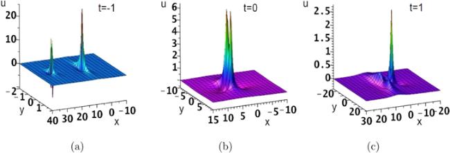
Figure 2. Evolution plots of the two-lump solution ( |
Higher-order lump solution. For the fixed parameters μ1 and ν1 (${\nu }_{1}={\mu }_{1}^{* }$), we can derive the Nth-order lump solution by making use of the higher-order derivatives of equation (
$\begin{eqnarray}u=2{\partial }_{x}^{2}\mathrm{ln}\widehat{{\rm{\Delta }}},\end{eqnarray}$
where $\begin{eqnarray*}\begin{array}{rcl}\widehat{{\rm{\Delta }}} & = & {\left({\widehat{{\rm{\Delta }}}}_{{ij}}\right)}_{N\times N}={\left(\displaystyle \frac{{\partial }^{i+j}{\rm{\Omega }}(\mu ,\nu )}{\partial {\mu }^{j}\partial {\nu }^{i}}\left|{}_{\mu ={\mu }_{1},\nu ={\nu }_{1}}\right.\right)}_{N\times N},\\ 1 & \leqslant & i,j\leqslant N.\end{array}\end{eqnarray*}$
Thus, the second-order lump solution can be represented in the following determinant form $\begin{eqnarray}\begin{array}{l}u[-2,+2]=2{\partial }_{x}^{2}\\ \times \mathrm{ln}\left|\begin{array}{cc}\tfrac{{\partial }^{2}{\rm{\Omega }}(\mu ,\nu )}{\partial \mu \partial \nu }{| }_{\mu ={\mu }_{1},\nu ={\nu }_{1}} & \tfrac{{\partial }^{3}{\rm{\Omega }}(\mu ,\nu )}{\partial {\mu }^{2}\partial \nu }{| }_{\mu ={\mu }_{1},\nu ={\nu }_{1}}\\ \tfrac{{\partial }^{3}{\rm{\Omega }}(\mu ,\nu )}{\partial \mu \partial {\nu }^{2}}{| }_{\mu ={\mu }_{1},\nu ={\nu }_{1}} & \tfrac{{\partial }^{4}{\rm{\Omega }}(\mu ,\nu )}{\partial {\mu }^{2}\partial {\nu }^{2}}{| }_{\mu ={\mu }_{1},\nu ={\nu }_{1}}\end{array}\right|.\end{array}\end{eqnarray}$
We exhibit in figure 3 the evolution plots of the second-order lump solution by choosing specific parameters. One can find that the maximum amplitude of the second-order lump solution is much larger than the two-lump solution.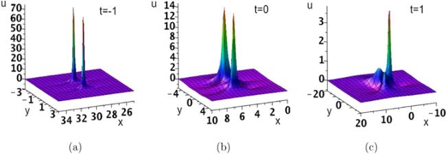
Figure 3. Evolution plots of the second-order lump solution ( |
General lump-soliton interaction solution. At this stage, we can end up with the (N1, N2) lump-soliton interaction solution
$\begin{eqnarray}\begin{array}{rcl}u & = & 2{\partial }_{x}^{2}\mathrm{ln}\widetilde{{\rm{\Delta }}},\\ \ \ \widetilde{{\rm{\Delta }}} & = & {\left({\widetilde{{\rm{\Delta }}}}_{{ij}}\right)}_{N\times N},\\ {\widetilde{{\rm{\Delta }}}}_{{ij}} & = & \left\{\begin{array}{l}{\rm{\Omega }}(\mu ,\nu ){| }_{\mu ={\mu }_{j},\nu ={\nu }_{i}},C={\delta }_{{ij}},1\leqslant i,j\leqslant {N}_{2},\\ \tfrac{\partial }{\partial \nu }{\rm{\Omega }}(\mu ,\nu ){| }_{\mu ={\mu }_{j},\nu ={\nu }_{i}},{N}_{2}+1\leqslant i\leqslant {N}_{1}+{N}_{2},1\leqslant j\leqslant {N}_{2},\\ \tfrac{\partial }{\partial \mu }{\rm{\Omega }}(\mu ,\nu ){| }_{\mu ={\mu }_{j},\nu ={\nu }_{i}},1\leqslant i\leqslant {N}_{2},{N}_{2}+1\leqslant j\leqslant {N}_{1}+{N}_{2},\\ \tfrac{{\partial }^{2}}{\partial \mu \partial \nu }{\rm{\Omega }}(\mu ,\nu ){| }_{\mu ={\mu }_{j},\nu ={\nu }_{i}},{N}_{2}+1\leqslant i,j\leqslant {N}_{1}+{N}_{2},\end{array}\right.\end{array}\end{eqnarray}$
and the (N1th-order, N2) lump-soliton interaction solution $\begin{eqnarray}\begin{array}{rcl}u & = & 2{\partial }_{x}^{2}\mathrm{ln}\overline{{\rm{\Delta }}},\\ \overline{{\rm{\Delta }}} & = & {\left({\overline{{\rm{\Delta }}}}_{{ij}}\right)}_{N\times N},\\ {\overline{{\rm{\Delta }}}}_{{ij}} & = & \left\{\begin{array}{l}{\rm{\Omega }}(\mu ,\nu ){| }_{\mu ={\mu }_{j},\nu ={\nu }_{i}},C={\delta }_{{ij}},1\leqslant i,j\leqslant {N}_{2},\\ \tfrac{{\partial }^{i-{N}_{2}}}{\partial {\nu }^{i-{N}_{2}}}{\rm{\Omega }}(\mu ,\nu ){| }_{\mu ={\mu }_{j},\nu ={\nu }_{{N}_{2}+1}},{N}_{2}+1\leqslant i\leqslant {N}_{1}+{N}_{2},1\leqslant j\leqslant {N}_{2},\\ \tfrac{{\partial }^{j-{N}_{2}}}{\partial {\mu }^{{}^{j-{N}_{2}}}}{\rm{\Omega }}(\mu ,\nu ){| }_{\mu ={\mu }_{{N}_{2}+1},\nu ={\nu }_{i}},1\leqslant i\leqslant {N}_{2},{N}_{2}+1\leqslant j\leqslant {N}_{1}+{N}_{2},\\ \tfrac{{\partial }^{i+j-2{N}_{2}}}{\partial {\mu }^{j-{N}_{2}}\partial {\nu }^{i-{N}_{2}}}{\rm{\Omega }}(\mu ,\nu ){| }_{\mu ={\mu }_{{N}_{2}+1},\nu ={\nu }_{{N}_{2}+1}},{N}_{2}+1\leqslant i,j\leqslant {N}_{1}+{N}_{2},\end{array}\right.\end{array}\end{eqnarray}$
where N1+N2 = N. For N1 = N2 = 1, we have $\begin{eqnarray}\begin{array}{l}u[-2,+2]=2{\partial }_{x}^{2}\\ \times \,\mathrm{ln}\left|\begin{array}{cc}{\rm{\Omega }}(\mu ,\nu ){| }_{\mu ={\mu }_{1},\nu ={\nu }_{1},C=1} & \tfrac{\partial {\rm{\Omega }}(\mu ,\nu )}{\partial \mu }{| }_{\mu ={\mu }_{2},\nu ={\nu }_{1}}\\ \tfrac{\partial {\rm{\Omega }}(\mu ,\nu )}{\partial \nu }{| }_{\mu ={\mu }_{1},\nu ={\nu }_{2}} & \tfrac{{\partial }^{2}{\rm{\Omega }}(\mu ,\nu )}{\partial \mu \partial \nu }{| }_{\mu ={\mu }_{2},\nu ={\nu }_{2}}\end{array}\right|.\end{array}\end{eqnarray}$
The interactions between one lump and one soliton separating or merging with each other described by equation (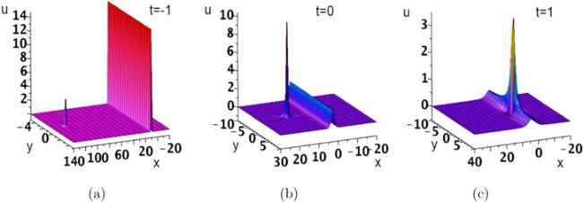
Figure 4. Interactions between one lump and one soliton described by equation ( |
5. Conclusion
In conclusion, we presented the Lax pair and conjugate Lax pair for the variable coefficient KP equation through the Painlevé analysis. We then constructed the N-fold binary DT in the compact determinant representation. As an application, we derived the arbitrary-order multi-lump, higher-order lump and general lump-soliton interaction solutions. Typically, we showed the evolution plots of the one-lump solution, two-lump solution, second-order lump solution and interactions between one lump and one soliton.