


1. Introduction
Over the past forty decades, some evidence can prove that we can get the quantum of space–time geometry connecting with classical thermodynamic theory by the black hole thermodynamics. The related work originated from Hawking and Bekenstein [1–5] which first defined the entropy and temperature for a black hole. Since then, the thermodynamic properties of the black hole have been widely studied [6–11]. In 1983, Hawking and Page [12] found a certain phase transition between the Schwarzschild black hole and thermal state, i.e. Hawking–Page phase transition. This has caused widespread attention about the thermodynamic properties of AdS black holes. Then, Chamblin et al [13, 14] studied the phase transition of the RN-AdS black hole and revealed the close relationship between the charged AdS black hole and the liquid–gas system.
In the original form of the first thermodynamical law for a black hole, there takes the black hole mass M to interpret as the internal energy U. And the first thermodynamical law for the charged rotating black hole is ${\rm{d}}{M}={T}{\rm{d}}{S}+{\rm{d}}{J}+{\rm{d}}{Q}$, where the entropy S and the temperature T dependent on the area of the event horizon A and the surface gravity κ, respectively. Ω is its angular velocity conjugate to the angular momentum J, and its electric potential Φ is conjugated to the charge Q.
Somewhat more recently the thermodynamics of AdS black hole has been widely studied in the extended phase space, in which the cosmological constant plays the role as the thermodynamic pressure [15–18] $P=\tfrac{-{\rm{\Lambda }}}{8\pi }$ and its conjugate quantity is the thermodynamic volume. So we know that the black hole mass M is more like the enthalpy H rather than the internal energy U. Moreover we regard the cosmological constant as the thermodynamic pressure in first thermodynamical law, which makes it match the Smarr relation. The expansion VdP in the first law led to a more interesting development of the black hole thermodynamics. Since then, many studies about the black hole phase structure analogous to Van der Waals (VdW) liquid–gas systems in the extended phase space have been founded in different AdS black holes [19–23].
The recent research on the black hole thermodynamics was holographic engine [24, 25]. It naturally makes the classic heat engine be introduced into the black hole thermodynamics because of the thermodynamic volume and pressure, which are defined in the extended phase space, are both dynamical variables and we can calculate mechanical work via the VdP term [24]. In this paper we give a brief review on the heat engine in curved black hole ground. The heat engine was constructed by defined a heat cycle which is a closed path in the P–v plane. During the working process, it was allowed the input of the amount of heat QH from warmer reservoirs (correspond to the temperature TH), and the output of the amount of heat QC into colder reservoirs (correspond to the temperature TC, TH > TC). A total mechanical work W is defined by W = QC − QH . So the efficiency of the heat engine is defined as $\eta =\tfrac{W}{{Q}_{H}}=1-\tfrac{{Q}_{C}}{{Q}_{H}}$. In the classic heat engines, it is well known that the efficiency of the Carnot heat engine is $\eta =1-\tfrac{{T}_{C}}{{T}_{H}}$. The holographic engine is described by the conformal field theory in the boundary [26]. And Johnson [24] creatively used the charged AdS black hole as heat engine working substances to construct a holographic heat engine and he calculated the heat engine efficiency. Then, the holographic heat engines were investigated in different black hole backgrounds, such as the Born–Infeld black hole [27], the 3-dimensional charged BTZ black hole [28], the rotating black hole [29] and the accelerating AdS black hole [30].
We all know that, under general conditions, the collapsed object with sufficient mass will undergo continuous gravitational collapse, leading to the formation of curvature singularities. This concept is called singularity theorems of Hawking and Penrose [31]. In the curvature singularity, there no longer exists the space–time and the physical properties. So we should use the quantum gravity to solve this problem. However, the quantum gravity is not yet fully mature, therefore some black holes without curvature singularity called ‘regular’ black holes are very interesting for physic scientists to investigate in the whole world. In 1968, Bardeen [32] acquired a black hole solution without the singularity and this is the well known black hole called Bardeen black hole. And so many studies on the physical properties of the regular black hole have been done. Such as the phase transition and geometrothermodynamics of regular electrically charged black hole in nonlinear electrodynamics theory coupled to general relativity have been investigated in [33]. In [34, 35], some authors have investigated the thermodynamics and geometrothermodynamics of regular Bardeen AdS black hole with a quintessence. Rajani [36] has made the Bardeen AdS black hole as work substance constructed a heat engine and also calculated the heat efficiency. In the present work, we will focus on the thermodynamics and the heat engine in the background of Bardeen AdS black hole in the Einstein–Gauss–Bonnet (EGB) theory. In [37, 38] Nam et al has investigated the extended phase space thermodynamics of regular charged AdS black hole in GaussCBonnet gravity, and charged AdS black holes in Gauss–Bonnet gravity and nonlinear electrodynamics. What is different from the work of Nam is that we are looking at higher dimensions. The EGB theory makes a generalization of Einstein’s general relativity to the higher dimensions by the heterotic string theory [39, 40]. The first EGB black hole solution was obtained by Boulware and Deser, and at r = 0 it is similar to its general relativity counterpart with a curvature singularity [41]. And the Bardeen AdS black hole in the EGB theory was obtained by Kumar and Singh [42].
This paper is organized as follows. In section 2 , we take a bright review of the basic thermodynamics properties of the Bardeen EGB AdS black hole. In section 3 , we study the P–v criticality of the Bardeen EGB-AdS black hole and draw the P–v diagram. In section 4 , the heat engine efficiency of this system is studied. The results and discussions are presented in section 5 .
2. The Bardeen AdS blackhole in the EGB theory
The action of the EGB gravity with the negative cosmological constant coupled to nonlinear electrodynamics [43] reads:
$\begin{eqnarray}\begin{array}{rcl}{{ \mathcal I }}_{G} & = & \displaystyle \frac{1}{2}{\displaystyle \int }_{M}{{\rm{d}}}^{D}x\sqrt{-g}\left[R+\alpha {{ \mathcal L }}_{{\rm{GB}}}\right.\\ & & \left.+\displaystyle \frac{(D-1)(D-2)}{{l}^{2}}+{ \mathcal L }(F)\right],\end{array}\end{eqnarray}$
where Λ = −(D − 1)(D − 2)/2l2 is the cosmological constant and α is the Gauss–Bonnet coupling coefficient with dimension [length]2. The discussion in our paper will take place when $\alpha \geqslant 0$ [44, 45]. The Gauss–Bonnet term (${ \mathcal L }({\rm{GB}})={R}_{\mu \nu \gamma \delta }{R}^{\mu \nu \gamma \delta }-4{R}_{\mu \nu }{R}^{\mu \nu }+{R}^{2}$) in four-dimension is a topological term, so the study is in over five-dimension [42]. The ${ \mathcal L }(F)$ is nonlinear electrodynamics function of Lorentz invariant, $F={F}_{\mu \nu }{F}^{\mu \nu }/4$, where ${F}_{\mu \nu }=2{{\rm{\nabla }}}_{{[}_{\mu }{A}_{\nu }]}$ (Aν is gauge potential).From [42] we get the Lagrangian density of the matter field
$\begin{eqnarray}{ \mathcal L }(F)=\displaystyle \frac{1}{4{{se}}^{2}}{\left[\displaystyle \frac{\sqrt{2{e}^{2}F}}{1+\sqrt{2{e}^{2}F}}\right]}^{\displaystyle \frac{2D-3}{D-2}},\end{eqnarray}$
with $\begin{eqnarray}s=\left\{\begin{array}{ll}\displaystyle \frac{{{e}}^{D-3}}{(D-1)\mu {{\prime} }^{D-3}}, & D={\rm{even}},\\ \displaystyle \frac{{{e}}^{D-3}}{(D-3)\mu {{\prime} }^{D-3}}, & D={\rm{odd}}.\end{array}\right.\end{eqnarray}$
In D-dimensional space–time we assume the metric as
$\begin{eqnarray}{{\rm{d}}{s}}^{2}=-f(r){{\rm{d}}{t}}^{2}+\displaystyle \frac{1}{f(r)}{{\rm{d}}{r}}^{2}+{r}^{2}{\tilde{\gamma }}_{{ij}}{{\rm{d}}{x}}^{i}{{\rm{d}}{x}}^{j},\end{eqnarray}$
where the ${\tilde{\gamma }}_{{ij}}$ is the metric of (D − 2)-dimensional constant curvature space k = 0, 1 or −1. And the solution of above action has been obtained as [42]: $\begin{eqnarray}\begin{array}{l}{f}_{\pm }(r)=1+\displaystyle \frac{{r}^{2}}{2\tilde{\alpha }}(1\pm \sqrt{\displaystyle \frac{4\tilde{\alpha }\mu ^{\prime} }{{\left({r}^{D-2}+{e}^{D-2}\right)}^{\tfrac{D-1}{D-2}}-\tfrac{4\tilde{\alpha }}{{l}^{2}}}}),\\ D\geqslant 5\end{array}\end{eqnarray}$
with $\tilde{\alpha }=(D-3)(D-4)\alpha $, e is the charge constant and $\mu ^{\prime} $ is the mass of the black hole, which is related to the Arnowitt–Deser–Misner mass M with relation as [46] $\begin{eqnarray}\mu ^{\prime} =\displaystyle \frac{16\pi M}{(D-2){V}_{D-2}}\ {\rm{with}}\ {\omega }_{D-2}=\displaystyle \frac{2{\pi }^{\tfrac{D-1}{2}}}{{\rm{\Gamma }}(D-1)/2}.\end{eqnarray}$
There are two cases of the black hole solutions which correspond to the sign (±) in front of the square in the equation (5 ). Here we only discuss the case for sign $(-)$. The mass, the Hawking temperature, and the entropy were obtained in [42] as
$\begin{eqnarray}M=\displaystyle \frac{(D-2){\omega }_{D-2}{r}_{+}^{D-3}}{16\pi }\left[\left(1+\displaystyle \frac{\tilde{\alpha }}{{r}_{+}^{2}}+\displaystyle \frac{{r}_{+}^{2}}{{l}^{2}}\right){\left(1+\displaystyle \frac{{e}^{D-2}}{{r}_{+}^{D-2}}\right)}^{\displaystyle \frac{D-1}{D-2}}\right]\end{eqnarray}$
$\begin{eqnarray}T=\displaystyle \frac{1}{4\pi {r}_{+}}\left[\displaystyle \frac{(D-3){r}_{+}^{2}+(D-5)\tilde{\alpha }-\tfrac{2{e}^{D-2}}{{r}_{+}^{D-2}}({r}_{+}^{2}+2\tilde{\alpha })+\tfrac{D-1}{{l}^{2}}{r}_{+}^{4}}{\left({r}_{+}^{2}+2\tilde{\alpha })(1+\tfrac{{e}^{D-2}}{{r}_{+}^{D-2}}\right)}\right]\end{eqnarray}$
$\begin{eqnarray}\begin{array}{rcl}S & = & \displaystyle \frac{(D-1){\omega }_{D-2}{\left(1+\tfrac{{e}^{D-2}}{{r}_{+}^{D-2}}\right)}^{\tfrac{D-1}{D-2}}{r}_{+}^{D-2}}{4}\\ & & \times \left[(D-4)\displaystyle \frac{{r}_{+}^{D-2}}{{e}^{D-2}}{H}_{1}+(D-3)\left[\displaystyle \frac{2\tilde{\alpha }}{{r}_{+}^{2}}{H}_{2}-(D-4){H}_{3}\right]\right.\\ & & \left.-(D-3)(D-4)\tilde{\alpha }\displaystyle \frac{{e}^{D-2}}{{r}_{+}^{D}}{H}_{4}\right]\end{array}\end{eqnarray}$
with $\begin{eqnarray}\begin{array}{l}{H}_{1}{=}_{2}{F}_{1}\left[1,2,\displaystyle \frac{-(2D-5)}{(D-2)},-\displaystyle \frac{{r}_{+}^{D-2}}{{e}^{D-2}}\right],\\ {H}_{2}{=}_{2}{F}_{1}\left[1,\displaystyle \frac{3}{(D-2)},\displaystyle \frac{2}{(D-2)},-\displaystyle \frac{{e}^{D-2}}{{r}_{+}^{D-2}}\right],\\ {H}_{3}{=}_{2}{F}_{1}\left[1,1,\displaystyle \frac{(D-3)}{(D-2)},-\displaystyle \frac{{r}_{+}^{D-2}}{{e}^{D-2}}\right],\\ {H}_{4}{=}_{2}{F}_{1}\left[1,\displaystyle \frac{(D+1)}{(D-2)},\displaystyle \frac{D}{(D-2)},-\displaystyle \frac{{e}^{D-2}}{{r}_{+}^{D-2}}\right].\end{array}\end{eqnarray}$
With above quantities we can get the first law of thermodynamics as [47] $\begin{eqnarray}{\rm{d}}{M}={T}{\rm{d}}{S}+{\rm{\Phi }}{\rm{d}}{e}+{\rm{\Psi }}{\rm{d}}\alpha .\end{eqnarray}$
In the extended phase space, it is necessary to consider the cosmological constant plays the role as the thermodynamic pressure $P=\tfrac{-{\rm{\Lambda }}}{8\pi }$, moreover the mass of black hole regarded as the enthalpy. As a consequence the extended first law of thermodynamics is
$\begin{eqnarray}{\rm{d}}{M}={T}{\rm{d}}{S}+{\rm{\Phi }}{\rm{d}}{e}+{V}{\rm{d}}{P}+{\rm{\Psi }}{\rm{d}}\alpha ,\end{eqnarray}$
where S is the entropy of the black hole, Φ is the potential and e is the charge constant and α is Gauss–Bonnet parameter whose conjugate is ψ. And the Smarr relation is $\begin{eqnarray}(D-3)M=(D-2){TS}+{\rm{\Phi }}e-2{PV}+{\rm{\Psi }}\alpha ,\end{eqnarray}$
3. P–v criticality of Bardeen AdS-EGB black hole
In this section, we will discuss the P–v criticality of the Bardeen EGB-AdS black hole. We consider the cosmological constant as the thermodynamic pressure
$\begin{eqnarray}P=-\displaystyle \frac{{\rm{\Lambda }}}{8\pi }=\displaystyle \frac{(D-1)(D-2)}{16\pi {l}^{2}}.\end{eqnarray}$
Inputting equation (14 ) into (7 ), we can get the mass M as a function of pressure P15 ) reduces to the mass of D-dimensional Bardeen-AdS black hole [48] in the limit $\alpha \to 0$ as
$\begin{eqnarray}\begin{array}{l}M({r}_{+},P)=\displaystyle \frac{(D-2){\omega }_{D-2}{r}_{+}^{D-3}}{16\pi }\left[\left(1+\displaystyle \frac{\tilde{\alpha }}{{r}_{+}^{2}}\right.\right.\\ \ \ \left.\left.+\displaystyle \frac{16\pi P}{(D-1)(D-2)}{r}_{+}^{2}\right){\left(1+\displaystyle \frac{{e}^{D-2}}{{r}_{+}^{D-2}}\right)}^{\tfrac{D-1}{D-2}}\right].\end{array}\end{eqnarray}$
The mass expression ( $\begin{eqnarray}\begin{array}{l}M({r}_{+},P)=\displaystyle \frac{(D-2){\omega }_{D-2}{r}_{+}^{D-3}}{16\pi }\\ \ \times \,\left[\left(1+\displaystyle \frac{16\pi P}{(D-1)(D-2)}{r}_{+}^{2}\right){\left(1+\displaystyle \frac{{e}^{D-2}}{{r}_{+}^{D-2}}\right)}^{\tfrac{D-1}{D-2}}\right]\end{array}\end{eqnarray}$
we recover the mass of Schwarzschild–Tangherlini–AdS black holes in higher dimensions [49] when e = 0, α = 0, and we obtained the mass for the EGB-AdS black hole [50, 51] in the case of no charge (e = 0) $\begin{eqnarray}\begin{array}{l}M({r}_{+},P)=\displaystyle \frac{(D-2){\omega }_{D-2}{r}_{+}^{D-3}}{16\pi }\\ \ \ \ \times \,\left(1+\displaystyle \frac{\tilde{\alpha }}{{r}_{+}^{2}}+\displaystyle \frac{16\pi P}{(D-1)(D-2)}{r}_{+}^{2}\right).\end{array}\end{eqnarray}$
The Hawking temperature T as a function of pressure P can be determined by inputting equation (14 ) into (8 )18 ) reduces to the temperature of D-dimensional Bardeen-AdS black hole [48]
$\begin{eqnarray}\begin{array}{l}T({r}_{+},P)\\ =\displaystyle \frac{1}{4\pi {r}_{+}}\left[\displaystyle \frac{(D-3){r}_{+}^{2}+(D-5)\tilde{\alpha }-\tfrac{2{e}^{D-2}}{{r}_{+}^{D-2}}({r}_{+}^{2}+2\tilde{\alpha })+\tfrac{16\pi P}{D-2}{r}_{+}^{4}}{\left({r}_{+}^{2}+2\tilde{\alpha })(1+\tfrac{{e}^{D-2}}{{r}_{+}^{D-2}}\right)}\right].\end{array}\end{eqnarray}$
The temperature expression ( $\begin{eqnarray}T({r}_{+},P)=\displaystyle \frac{1}{4\pi {r}_{+}}\left[\displaystyle \frac{(D-3){r}_{+}^{2}-\tfrac{2{e}^{D-2}}{{r}_{+}^{D-2}}{r}_{+}^{2}+\tfrac{16\pi P}{D-2}{r}_{+}^{4}}{{r}_{+}^{2}(1+\tfrac{{e}^{D-2}}{{r}_{+}^{D-2}})}\right].\end{eqnarray}$
Solving (18 ), we can get21 ) Schwarzschild–Tangherlini–AdS black holes in higher dimensions [49].
$\begin{eqnarray}\begin{array}{l}P({r}_{+},T)=\displaystyle \frac{D-2}{16\pi {r}_{+}^{4}}\left[4\pi {r}_{+}T({r}_{+}^{2}+2\tilde{\alpha })\left(1+\displaystyle \frac{{e}^{D-2}}{{r}_{+}^{D-2}}\right)\right.\\ \ \ \left.-(D-3){r}_{+}^{2}-(D-5)\tilde{\alpha }+\displaystyle \frac{2{e}^{D-2}}{{r}_{+}^{D-2}}({r}_{+}^{2}+2\tilde{\alpha })\right].\end{array}\end{eqnarray}$
We reduce the state obtained for EGB-AdS black hole [52] when e = 0 $\begin{eqnarray}\begin{array}{rcl}P({r}_{+},T) & = & \displaystyle \frac{D-2}{16\pi {r}_{+}^{4}}\left[4\pi {r}_{+}T({r}_{+}^{2}+2\tilde{\alpha })\right.\\ & & \left.-(D-3){r}_{+}^{2}-(D-5)\tilde{\alpha }\right]\end{array}\end{eqnarray}$
when both e and α tend to zero, the equation of state ( $\begin{eqnarray}P({r}_{+},T)=\displaystyle \frac{D-2}{4\pi {r}_{+}}-\displaystyle \frac{(D-3)(D-2)}{16\pi {r}_{+}^{2}}.\end{eqnarray}$
Then we can calculate the critical value by equation (21 )
$\begin{eqnarray}\displaystyle \frac{\partial P}{\partial {r}_{+}}=0,\displaystyle \frac{{\partial }^{2}P}{{\partial }^{2}{r}_{+}}=0.\end{eqnarray}$
When the Bardeen parameter e = 0, the black hole reduces to D-dimensional EGB AdS black holes. When D = 5, the critical temperature Tc, the critical volume rc and critical pressure Pc of the 5-dimensional Gauss–Bonnet black hole [52] are
$\begin{eqnarray}{T}_{c}=\displaystyle \frac{1}{\pi \sqrt{24\tilde{\alpha }}}\ {v}_{c}=\displaystyle \frac{4}{3}\sqrt{6\tilde{\alpha }}\ {P}_{c}=\displaystyle \frac{1}{8\pi \tilde{\alpha }}.\end{eqnarray}$
Using the critical quantities, we can calculate $\tfrac{{P}_{c}{v}_{c}}{{T}_{c}}=\tfrac{1}{3}$.Because the original equation (23 ) is too complicated to be explicitly expressed, in this work we employ the numerical method to solve it. According to the boundary conditions of the black hole, we take different Bardeen parameter e (e under the critical value of eE) in different dimensions, respectively. The example numerical results are shown in table 1. From the numerical results, we can obtain the relationship between the critical volume, the critical radius and the critical pressure. In the table, we can find that the ratio ($\tfrac{{P}_{c}{v}_{c}}{{T}_{c}}$) of this black hole system is smaller but very close to the ratio relation of VdW system in the 5-dimensions. To further investigate this relationship, we calculated the pressure function of volume and temperature.
Table 1. The critical thermodynamic quantity for different dimensions with fixed the Bardeen parameter e and the Gauss–Bonnet parameter α. |
| α = 0.1 | α = 0.2 | |||||||
|---|---|---|---|---|---|---|---|---|
| Dimensions | e | rc | Tc | Pc | rc | Tc | Pc | |
| D = 5 | 0.4 | 1.552 62 | 0.122 67 | 0.021 74 | 0.3 | 1.726 83 | 0.098 68 | 0.014 88 |
| 0.3 | 1.362 14 | 0.132 42 | 0.026 08 | 0.2 | 1.612 69 | 0.101 36 | 0.016 53 | |
| D = 6 | 0.4 | 1.593 99 | 0.139 94 | 0.028 78 | 0.3 | 1.820 07 | 0.102 15 | 0.016 15 |
| 0.3 | 1.424 47 | 0.142 87 | 0.030 92 | 0.2 | 1.685 00 | 0.102 59 | 0.016 46 | |
| D = 7 | 0.4 | 0.997 62 | 0.160 08 | 0.057 61 | 0.3 | 0.649 34 | 0.161 21 | 0.417 76 |
| 0.3 | 0.683 09 | 0.181 73 | 0.170 00 | 0.2 | 0.421 98 | 0.224 74 | 2.510 64 | |
| D = 8 | 0.4 | 0.777 04 | 0.217 59 | 0.365 39 | 0.3 | 0.559 88 | 0.257 50 | 2.726 02 |
| 0.3 | 0.568 60 | 0.270 31 | 1.256 49 | 0.2 | 0.370 12 | 0.375 54 | 14.544 6 | |
According to the first law of thermodynamics equations (12 ) and (15 ), and taking r+ > >e, it is easily to obtain
$\begin{eqnarray}V={\left(\displaystyle \frac{\partial M}{\partial P}\right)}_{e,s}=\displaystyle \frac{{\omega }_{D-2}{r}_{+}^{D-1}}{(D-1)}.\end{eqnarray}$
Since we plan to compare the equation (21 ) with VdW equation, so we make the VdW equation expand with the inverse of specific volume v as21 ) as the similar form
$\begin{eqnarray}\begin{array}{l}P=\displaystyle \frac{T}{v-b}-\displaystyle \frac{a}{{v}^{2}}\approx \displaystyle \frac{T}{v}+\displaystyle \frac{{bT}}{{v}^{2}}+\displaystyle \frac{{b}^{2}T}{{v}^{3}}\\ \ \ \ +\ \displaystyle \frac{{b}^{3}T}{{v}^{4}}-\displaystyle \frac{a}{{v}^{2}}+o({v}^{-5}).\end{array}\end{eqnarray}$
At the same time, we expand the equation ( $\begin{eqnarray}\begin{array}{l}P({r}_{+},T)=\displaystyle \frac{{{Te}}^{D-2}{r}_{+}^{1-D}(D-2)}{4}+\displaystyle \frac{{{Te}}^{D-2}(D-2)}{2{r}_{+}^{D+1}}\\ \ \ \,\,+\ \displaystyle \frac{T(D-2)}{4{r}_{+}}+\displaystyle \frac{T\tilde{\alpha }(D-2)}{2{r}_{+}^{3}}\\ \,\,-\,\displaystyle \frac{D-2}{16{e}^{2}\pi {r}_{+}^{4+D}}\left(\tilde{\alpha }\left(D-5){e}^{2}{r}_{+}^{D}-4{e}^{D}{r}_{+}^{2}\right)\right.\\ \ \ \,\,\left.+\,\ {r}_{+}^{2}\left({e}^{2}{r}_{+}^{D}(D-3)-2{e}^{D}{r}_{+}^{2}\right)\right).\end{array}\end{eqnarray}$
Thus we can define the specific volume [49, 52, 53] as27 ) can read29 ) reduces to the state equation of the Schwarzschild–Tangherlini–AdS black holes in higher dimensions [49].
$\begin{eqnarray}v=\displaystyle \frac{4{{\ell }}^{D-2}}{D-2}{r}_{+}\end{eqnarray}$
taking ℓ as a unit, so equation ( $\begin{eqnarray}\begin{array}{rcl}P(v,T) & = & \displaystyle \frac{16}{\pi {\left(D-2\right)}^{3}{v}^{4}}\left[(D-2)T\pi v\right.\\ & & \times \left(\displaystyle \frac{{\left(D-2\right)}^{2}{v}^{2}}{16}+2\tilde{\alpha }\right)\left(1+\displaystyle \frac{{\left(4e\right)}^{D-2}}{{\left(D-2\right)}^{D-2}{v}^{D-2}}\right)\\ & & -(D-3)\displaystyle \frac{{\left(D-2\right)}^{2}{v}^{2}}{16}-(D-5)\tilde{\alpha }\\ & & \left.+\displaystyle \frac{2{\left(4e\right)}^{D-2}}{{\left(D-2\right)}^{D-2}{v}^{D-2}}\left(\displaystyle \frac{{\left(D-2\right)}^{2}{v}^{2}}{16}+4\tilde{\alpha }\right)\right]\end{array}\end{eqnarray}$
the equation (To investigate the thermodynamical critical properties of the Bardeen EGB-AdS black hole system which describes with the equation (29 ), we have simulated the state equation in figures 1 and 2 for different values of the Gauss–Bonnet parameter α. From the P–v diagram, we can intuitively see, when the parameter α changes from 0.1 to 0.2, the value of critical temperature decreases and the Bardeen EGB-AdS black hole conforms to the VdW system. But we should notice that $\tfrac{{P}_{c}{v}_{c}}{{T}_{c}}=0.369$ of the Bardeen EGB-AdS black hole system is between $\tfrac{{P}_{c}{v}_{c}}{{T}_{c}}=1/3=0.3333$ of the Gauss–Bonnet AdS black hole [52] and $\tfrac{{P}_{c}{v}_{c}}{{T}_{c}}=3/8=0.375$ of the VdW gas system in the 5-dimensions, because of Tc depends on the Bardeen parameter e and the Gauss–Bonnet parameter α.
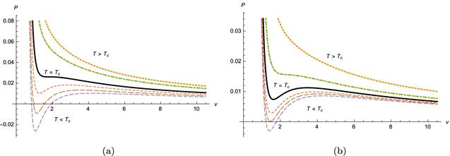
Figure 1. The criticality P–v diagram of the Bardeen-EGB-AdS black hole: (a) the dimension D = 5 case with fixed the Gauss–Bonnet parameter α = 0.1 and the Bardeen parameter e = 0.3; (b) the dimension D = 5 case with fixed the Gauss–Bonnet parameter α = 0.2 and the Bardeen parameter e = 0.3. |
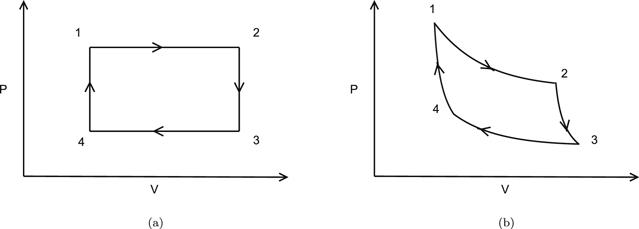
Figure 2. P–v diagram of thermodynamic cycles for the heat engine: (a) the rectangle cycle. Paths $1\to 2$ and $3\to 4$ are isobar. Paths $2\to 3$ and $4\to 1$ are isochoric. (b) The Carnot cycle. Paths $1\to 2$ and $3\to 4$ are isothermal. Paths $2\to 3$ and $4\to 1$ are adiabatic. |
4. Heat engine
In order to study the heat efficiency in the Bardeen EGB-AdS black hole space–time, we will follow a kind of the new heat engine that was constructed in [54]. We consider a rectangle cycle consisting of two isochores and two isobars in the P–v plane (see figure 2(a)). Subscripts 1, 2, 3, 4 of the physical quantities denote the four corresponding corners in the heat engine cycle in figure 2. From the equations (25 ) and (8 ), it is easy to obtain the entropy equation (9 ) as the function of the volume (defining by equation (25 )). We can conclude that specific heat at constant volume CV equals to zero. The isobar paths coincide with the adiabatic paths, which means no heat flows along the isobar.
To facilitate the calculation, we will take $D=5,{\omega }_{3}\,=2{\pi }^{2}$, and the work of done along the heat cycle is
$\begin{eqnarray}\begin{array}{rcl}W & = & \oint {P}{\rm{d}}{V}=({P}_{1}-{P}_{4})({v}_{2}-{v}_{1})\\ & = & \displaystyle \frac{{\pi }^{2}}{2}({P}_{1}-{P}_{4})\left({r}_{2}^{4}-{r}_{1}^{4}\right).\end{array}\end{eqnarray}$
Then, the magnitude of the input heat is described as
$\begin{eqnarray}\begin{array}{rcl}{Q}_{H} & = & {\displaystyle \int }_{{T}_{1}}^{{T}_{2}}{C}_{P}({P}_{1},T){\rm{d}}{T}={\displaystyle \int }_{{S}_{1}}^{{S}_{2}}P({P}_{1},T)\left(\displaystyle \frac{\partial T}{\partial S}\right){\rm{d}}{S}\\ & = & {\displaystyle \int }_{{S}_{1}}^{{S}_{2}}{T}{\rm{d}}{S}={\displaystyle \int }_{{H}_{1}}^{{H}_{2}}={M}_{2}-{M}_{1}.\end{array}\end{eqnarray}$
Combining with equation (15 ), QH can be obtained as
$\begin{eqnarray}{Q}_{H}=\displaystyle \frac{3\pi {r}_{+}^{2}}{8}{\left[\left(1+\displaystyle \frac{2\alpha }{{r}_{+}^{2}}+\displaystyle \frac{4\pi {{\Pr }}_{+}^{2}}{3}\right)\left.{\left(1+\displaystyle \frac{{e}^{3}}{{r}_{+}^{3}}\right)}^{\tfrac{4}{3}}\right]\right|}_{{r}_{1}}^{{r}_{2}}.\end{eqnarray}$
Thus, the heat engine efficiency is given by
$\begin{eqnarray}\eta =\displaystyle \frac{W}{{Q}_{H}}=\displaystyle \frac{4\pi }{3}\displaystyle \frac{({P}_{1}-{P}_{4})({r}_{2}^{4}-{r}_{1}^{4})}{{r}_{+}^{2}{\left[\left(1+\tfrac{2\alpha }{{r}_{+}^{2}}+\tfrac{4\pi {{\Pr }}_{+}^{2}}{3}\right)\left.{\left(1+\tfrac{{e}^{3}}{{r}_{+}^{3}}\right)}^{\tfrac{4}{3}}\right]\right|}_{{r}_{1}}^{{r}_{2}}}\end{eqnarray}$
and in the large-horizon regime ${r}_{+}\gt \gt e$ where the correction of e for the entropy be ignored, then the entropy turns to $\begin{eqnarray}S=\displaystyle \frac{{\pi }^{2}{r}_{+}}{2}(12\alpha +{r}_{+}^{2}).\end{eqnarray}$
From equations (33 ) and (34 ), we can obtain the efficiency as function of the pressure and the entropy
$\begin{eqnarray}\eta =\displaystyle \frac{W}{{Q}_{H}}=\displaystyle \frac{4\pi }{3}\displaystyle \frac{({P}_{1}-{P}_{4})\left(\tfrac{{\left[{\left({S}_{2}+\sqrt{{S}_{2}^{2}+64{\pi }^{4}{\alpha }^{3}}\right)}^{\tfrac{2}{3}}-4{\pi }^{\tfrac{4}{3}}\alpha \right]}^{4}}{{\pi }^{\tfrac{8}{3}}{\left({S}_{2}+\sqrt{{S}_{2}^{2}+64{\pi }^{4}{\alpha }^{3}}\right)}^{\tfrac{4}{3}}}-\tfrac{{\left[{\left({S}_{1}+\sqrt{{S}_{1}^{2}+64{\pi }^{4}{\alpha }^{3}}\right)}^{\tfrac{2}{3}}-4{\pi }^{\tfrac{4}{3}}\alpha \right]}^{4}}{{\pi }^{\tfrac{8}{3}}{\left({S}_{1}+\sqrt{{S}_{1}^{2}+64{\pi }^{4}{\alpha }^{3}}\right)}^{\tfrac{4}{3}}}\right)}{\tfrac{{\left[{\left({S}_{2}+\sqrt{{S}_{2}^{2}+64{\pi }^{4}{\alpha }^{3}}\right)}^{\tfrac{2}{3}}-4{\pi }^{\tfrac{4}{3}}\alpha \right]}^{2}}{{\pi }^{\tfrac{4}{3}}{\left({S}_{2}+\sqrt{{S}_{2}^{2}+64{\pi }^{4}{\alpha }^{3}}\right)}^{\tfrac{2}{3}}}{A}_{1}{B}_{1}^{\tfrac{4}{3}}-\tfrac{{\left[{\left({S}_{1}+\sqrt{{S}_{1}^{2}+64{\pi }^{4}{\alpha }^{3}}\right)}^{\tfrac{2}{3}}-4{\pi }^{\tfrac{4}{3}}\alpha \right]}^{2}}{{\pi }^{\tfrac{4}{3}}{\left({S}_{1}+\sqrt{{S}_{1}^{2}+64{\pi }^{4}{\alpha }^{3}}\right)}^{\tfrac{2}{3}}}{A}_{2}{B}_{2}^{\tfrac{4}{3}}},\end{eqnarray}$
where $\begin{eqnarray*}\begin{array}{rcl}{A}_{1} & = & 1+\displaystyle \frac{2\alpha {\pi }^{\tfrac{4}{3}}{\left({S}_{2}+\sqrt{{S}_{2}^{2}+64{\pi }^{4}{\alpha }^{3}}\right)}^{\tfrac{2}{3}}}{{\left[{\left({S}_{2}+\sqrt{{S}_{2}^{2}+64{\pi }^{4}{\alpha }^{3}}\right)}^{\tfrac{2}{3}}-4{\pi }^{\tfrac{4}{3}}\alpha \right]}^{2}}\\ & & +\displaystyle \frac{4\pi P}{3}\displaystyle \frac{{\left[{\left({S}_{2}+\sqrt{{S}_{2}^{2}+64{\pi }^{4}{\alpha }^{3}}\right)}^{\tfrac{2}{3}}-4{\pi }^{\tfrac{4}{3}}\alpha \right]}^{2}}{{\pi }^{\tfrac{4}{3}}{\left({S}_{2}+\sqrt{{S}_{2}^{2}+64{\pi }^{4}{\alpha }^{3}}\right)}^{\tfrac{2}{3}}}\\ {B}_{1} & = & 1+\displaystyle \frac{{e}^{3}{\pi }^{2}({S}_{2}+\sqrt{{S}_{2}^{2}+64{\pi }^{4}{\alpha }^{3}})}{{\left[{\left({S}_{2}+\sqrt{{S}_{2}^{2}+64{\pi }^{4}{\alpha }^{3}}\right)}^{\tfrac{2}{3}}-4{\pi }^{\tfrac{4}{3}}\alpha \right]}^{3}}\\ {A}_{2} & = & 1+\displaystyle \frac{2\alpha {\pi }^{\tfrac{4}{3}}{\left({S}_{1}+\sqrt{{S}_{1}^{2}+64{\pi }^{4}{\alpha }^{3}}\right)}^{\tfrac{2}{3}}}{{\left[{\left({S}_{1}+\sqrt{{S}_{1}^{2}+64{\pi }^{4}{\alpha }^{3}}\right)}^{\tfrac{2}{3}}-4{\pi }^{\tfrac{4}{3}}\alpha \right]}^{2}}\\ & & +\displaystyle \frac{4\pi P}{3}\displaystyle \frac{{\left[{\left({S}_{1}+\sqrt{{S}_{1}^{2}+64{\pi }^{4}{\alpha }^{3}}\right)}^{\tfrac{2}{3}}-4{\pi }^{\tfrac{4}{3}}\alpha \right]}^{2}}{{\pi }^{\tfrac{4}{3}}{\left({S}_{1}+\sqrt{{S}_{1}^{2}+64{\pi }^{4}{\alpha }^{3}}\right)}^{\tfrac{2}{3}}}\\ {B}_{2} & = & 1+\displaystyle \frac{{e}^{3}{\pi }^{2}({S}_{1}+\sqrt{{S}_{1}^{2}+64{\pi }^{4}{\alpha }^{3}})}{{\left[{\left({S}_{1}+\sqrt{{S}_{1}^{2}+64{\pi }^{4}{\alpha }^{3}}\right)}^{\tfrac{2}{3}}-4{\pi }^{\tfrac{4}{3}}\alpha \right]}^{3}}.\end{array}\end{eqnarray*}$
To compare the maximum possible efficiency, i.e. the well-known Carnot heat engine, with our heat engine efficiency in this paper, we consider that the highest temperature TH and the lowest temperature TC in our cycle correspond to T2 and T4, respectively. So the efficiency of this Carnot heat engine is
$\begin{eqnarray}{\eta }_{c}\,=\,1-\displaystyle \frac{{T}_{C}}{{T}_{H}}\,=\,1-\displaystyle \frac{{r}_{1}}{{r}_{2}}\displaystyle \frac{\left[2{r}_{2}^{2}-\tfrac{2{e}^{3}}{{r}_{2}^{3}}({r}_{2}^{2}+4\alpha )+\tfrac{16\pi {P}_{1}}{3}{r}_{2}^{4}\right]({r}_{1}^{2}+4\alpha )(1+\tfrac{{e}^{3}}{{r}_{1}^{3}})}{\left[2{r}_{1}^{2}-\tfrac{2{e}^{3}}{{r}_{1}^{3}}({r}_{1}^{2}+4\alpha )+\tfrac{16\pi {P}_{4}}{3}{r}_{1}^{4}\right]({r}_{2}^{2}+4\alpha )\left(1+\tfrac{{e}^{3}}{{r}_{2}^{3}}\right)}.\end{eqnarray}$
Substituting equation (34 ) into the above equation, we can get
$\begin{eqnarray}{\eta }_{c}=1-\displaystyle \frac{{T}_{4}({P}_{4},{S}_{1})}{{T}_{2}({P}_{1},{S}_{2})}=1-\displaystyle \frac{\left[{\left({S}_{1}+\sqrt{{S}_{1}^{2}+64{\pi }^{4}{\alpha }^{3}}\right)}^{\tfrac{2}{3}}-4{\pi }^{\tfrac{4}{3}}\alpha \right]({\pi }^{\tfrac{2}{3}}{\left({S}_{2}+\sqrt{{S}_{2}^{2}+64{\pi }^{4}{\alpha }^{3}}\right)}^{\tfrac{1}{3}})}{\left[{\left({S}_{2}+\sqrt{{S}_{2}^{2}+64{\pi }^{4}{\alpha }^{3}}\right)}^{\tfrac{2}{3}}-4{\pi }^{\tfrac{4}{3}}\alpha \right]\left({\pi }^{\tfrac{2}{3}}{\left({S}_{1}+\sqrt{{S}_{1}^{2}+64{\pi }^{4}{\alpha }^{3}}\right)}^{\tfrac{1}{3}}\right)}\displaystyle \frac{({D}_{1}-{C}_{1}){B}_{2}{E}_{1}}{({D}_{2}-{C}_{2}){B}_{1}{E}_{2}},\end{eqnarray}$
where $\begin{eqnarray*}\begin{array}{rcl}{C}_{1} & = & \displaystyle \frac{2{e}^{3}{\pi }^{2}({S}_{2}+\sqrt{{S}_{2}^{2}+64{\pi }^{4}{\alpha }^{3}})}{{\left[{\left({S}_{2}+\sqrt{{S}_{2}^{2}+64{\pi }^{4}{\alpha }^{3}}\right)}^{\tfrac{2}{3}}-4{\pi }^{\tfrac{4}{3}}\alpha \right]}^{3}}\\ & & \times \left(\displaystyle \frac{{\left[{\left({S}_{2}+\sqrt{{S}_{2}^{2}+64{\pi }^{4}{\alpha }^{3}}\right)}^{\tfrac{2}{3}}-4{\pi }^{\tfrac{4}{3}}\alpha \right]}^{2}}{{\pi }^{\tfrac{4}{3}}{\left({S}_{2}+\sqrt{{S}_{2}^{2}+64{\pi }^{4}{\alpha }^{3}}\right)}^{\tfrac{2}{3}}}+4\alpha \right)\end{array}\end{eqnarray*}$
$\begin{eqnarray*}\begin{array}{rcl}{C}_{2} & = & \displaystyle \frac{2{e}^{3}{\pi }^{2}({S}_{1}+\sqrt{{S}_{1}^{2}+64{\pi }^{4}{\alpha }^{3}})}{{\left[{\left({S}_{1}+\sqrt{{S}_{1}^{2}+64{\pi }^{4}{\alpha }^{3}}\right)}^{\tfrac{2}{3}}-4{\pi }^{\tfrac{4}{3}}\alpha \right]}^{3}}\\ & & \times \left(\displaystyle \frac{{\left[{\left({S}_{1}+\sqrt{{S}_{1}^{2}+64{\pi }^{4}{\alpha }^{3}}\right)}^{\tfrac{2}{3}}-4{\pi }^{\tfrac{4}{3}}\alpha \right]}^{2}}{{\pi }^{\tfrac{4}{3}}{\left({S}_{1}+\sqrt{{S}_{2}^{1}+64{\pi }^{4}{\alpha }^{3}}\right)}^{\tfrac{2}{3}}}+4\alpha \right)\end{array}\end{eqnarray*}$
$\begin{eqnarray*}\begin{array}{rcl}{D}_{1} & = & 2\displaystyle \frac{{\left[{\left({S}_{2}+\sqrt{{S}_{2}^{2}+64{\pi }^{4}{\alpha }^{3}}\right)}^{\tfrac{2}{3}}-4{\pi }^{\tfrac{4}{3}}\alpha \right]}^{2}}{{\pi }^{\tfrac{4}{3}}{\left({S}_{2}+\sqrt{{S}_{2}^{2}+64{\pi }^{4}{\alpha }^{3}}\right)}^{\tfrac{2}{3}}}\\ & & +\displaystyle \frac{16\pi {P}_{1}}{3}\displaystyle \frac{{\left[{\left({S}_{2}+\sqrt{{S}_{2}^{2}+64{\pi }^{4}{\alpha }^{3}}\right)}^{\tfrac{2}{3}}-4{\pi }^{\tfrac{4}{3}}\alpha \right]}^{4}}{{\pi }^{\tfrac{8}{3}}{\left({S}_{2}+\sqrt{{S}_{2}^{2}+64{\pi }^{4}{\alpha }^{3}}\right)}^{\tfrac{4}{3}}}\end{array}\end{eqnarray*}$
$\begin{eqnarray*}\begin{array}{rcl}{D}_{2} & = & 2\displaystyle \frac{{\left[{\left({S}_{1}+\sqrt{{S}_{1}^{2}+64{\pi }^{4}{\alpha }^{3}}\right)}^{\tfrac{2}{3}}-4{\pi }^{\tfrac{4}{3}}\alpha \right]}^{2}}{{\pi }^{\tfrac{4}{3}}{\left({S}_{1}+\sqrt{{S}_{1}^{2}+64{\pi }^{4}{\alpha }^{3}}\right)}^{\tfrac{2}{3}}}\\ & & +\displaystyle \frac{16\pi {P}_{4}}{3}\displaystyle \frac{{\left[{\left({S}_{1}+\sqrt{{S}_{1}^{2}+64{\pi }^{4}{\alpha }^{3}}\right)}^{\tfrac{2}{3}}-4{\pi }^{\tfrac{4}{3}}\alpha \right]}^{4}}{{\pi }^{\tfrac{8}{3}}{\left({S}_{1}+\sqrt{{S}_{1}^{2}+64{\pi }^{4}{\alpha }^{3}}\right)}^{\tfrac{4}{3}}}\end{array}\end{eqnarray*}$
$\begin{eqnarray*}\begin{array}{rcl}{E}_{1} & = & \displaystyle \frac{{\left[{\left({S}_{1}+\sqrt{{S}_{1}^{2}+64{\pi }^{4}{\alpha }^{3}}\right)}^{\tfrac{2}{3}}-4{\pi }^{\tfrac{4}{3}}\alpha \right]}^{2}}{{\pi }^{\tfrac{4}{3}}{\left({S}_{1}+\sqrt{{S}_{1}^{2}+64{\pi }^{4}{\alpha }^{3}}\right)}^{\tfrac{2}{3}}}+4\alpha \\ {E}_{2} & = & \displaystyle \frac{{\left[{\left({S}_{2}+\sqrt{{S}_{2}^{2}+64{\pi }^{4}{\alpha }^{3}}\right)}^{\tfrac{2}{3}}-4{\pi }^{\tfrac{4}{3}}\alpha \right]}^{2}}{{\pi }^{\tfrac{4}{3}}{\left({S}_{2}+\sqrt{{S}_{2}^{2}+64{\pi }^{4}{\alpha }^{3}}\right)}^{\tfrac{2}{3}}}+4\alpha .\end{array}\end{eqnarray*}$
Because the analytical expresses of the heat engine efficiency η (see equation (35 )) and the ratio η/ηc (see equations (35 ) and (37 )) are so complicated, we numerically simulate them in figures 3 and 4, respectively. Figure 3 exhibits the efficiency for the Bardeen EGB-AdS black hole versus entropy S2, and the figure 4 exhibits the ratio between the efficiency and the Carnot efficiency versus entropy S2. Figure 3(a) shows the case with efficiency η versus entropy S2 for different values of the Bardeen parameter e with fixed Gauss–Bonnet parameter α and pressure P1, P4. From the figure 3(a), we can find that, for all values of Bardeen parameter e, the efficiency monotonically increases as the entropy S2 (corresponding to volume v2) grows and then tends to the saturation value. This means that the increase of volume difference between the small black hole (v1) and lager black hole (v2) will make the heat engine efficiency increase. And when the Bardeen parameter e becomes higher, the heat engine efficiency of the Bardeen EGB-AdS black hole will get lower. The figure 3(b) displays the case of the efficiency η versus entropy S2 with different values of the Gauss–Bonnet parameter α with fixed Bardeen parameter e and pressure P1, 4P4. And for all values of Gauss Bonnet parameter α, the curves grow similar as shown in the figure 3(a), but the different between figure 3(b) and (a) is as the Gauss Bonnet parameter α increases the efficiency of black hole will increase.
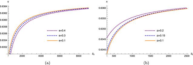
Figure 3. The efficiency of the heat engine versus the entropy for Bardeen EGB-AdS black hole. (a) The case for different Bardeen parameter e = 0.1, 0.3, 0.4 (from top to bottom) with the Gauss–Bonnet parameter α = 0.1, the pressure P1 = 4, P4 = 1 and the entropy S1 = 1. (b) The case for different Gauss–Bonnet parameter α = 0.2, 0.15, 0.1 (from top to bottom) with the Bardeen parameter e = 0.3, the pressure P1 = 4, P4 = 1 and the entropy S1 = 1. |
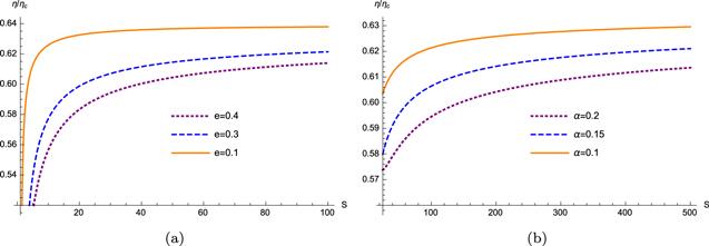
Figure 4. Ratio η/ηc between the rectangle cycle efficiency and the Carnot cycle efficiency versus entropy for the Bardeen-EGB-AdS black hole. (a) The case for different e = 0.1, 0.3, 0.4 (from top to bottom) with the Gauss–Bonnet parameter α = 0.1, the pressure P1 = 4, P4 = 1 and the entropy S1 = 1. (b) The case for different α = 0.1, 0.15, 0.2 (from top to bottom) with the Bardeen parameter e = 0.3, the pressure P1 = 4, P4 = 1 and the entropy S1 = 1. |
Figure 4 shows the ratio η/ηc against entropy S2 in different values of Bardeen parameter e with fixed Gauss Bonnet parameter α and Gauss–Bonnet α with fixed Bardeen parameter e, respectively. And from figures 4(a) and (b), we can see that the all curves monotonic grow rapidly firstly, then the efficiency reaches the saturation values after the certain value of entropy S2. For different Bardeen parameter e and Gauss–Bonnet parameter α, the rates of increment are different. Because the efficiency ratio η/ηc versus entropy S2 is bounded below 1, it coincides with the thermodynamical second law. In figure 4, the efficiency ratio η/ηc will both get lower when the Bardeen parameter e and the Gauss–Bonnet parameter α get higher.
5. Conclusion
In this paper, we have discussed the P–v criticality and the heat engine efficiency in the Bardeen EGB AdS black hole space–time. We have considered the cosmological constant as the thermodynamic pressure and thermodynamic volume as its conjugate quality to set up the extended phase space. We have studied the critical P–v plane and found that the Bardeen EGB-AdS black hole conform to VdW liquid–gas system in the extended phase space and the critical temperature decreases with the Gauss–Bonnet parameter α. Furthermore, we have noticed that $\tfrac{{P}_{c}{v}_{c}}{{T}_{c}}=0.369$ of the Bardeen EGB-AdS black hole system is between $\tfrac{{P}_{c}{v}_{c}}{{T}_{c}}=1/3=0.3333$ of the Gauss–Bonnet AdS black hole and $\tfrac{{P}_{c}{v}_{c}}{{T}_{c}}=3/8=0.375$ of the VdW gas system in the 5-dimensions.
Then we have constructed a heat engine by taking the Bardeen EGB-AdS black hole as a working substance, and we consider a rectangle heat cycle in the P–v plot. We have found that two cases, with different Bardeen parameter e and different Gauss– Bonnet parameter α both, have the same situation, i.e. as the entropy difference between small black hole S1 and larger black hole S2 increases, the heat engine efficiency will increase. Furthermore, as the Bardeen parameter e increases, the efficiency will decrease. However, for the the Gauss–Bonnet parameter α, the results are contrary. Then we have compared our efficiency results with the well-know Carnot heat engine efficiency, we have found the efficiency ratio η/ηc versus entropy S2 is bounded below 1, so it coincides with the thermodynamical second law.