In this paper, we give the general interaction solution to the (3+1)-dimensional Jimbo–Miwa equation. The general interaction solution contains the classical interaction solution. As an example, by using the generalized bilinear method and symbolic computation by using Maple software, novel interaction solutions under certain constraints of the (3+1)-dimensional Jimbo–Miwa equation are obtained. Via three-dimensional plots, contour plots and density plots with the help of Maple, the physical characteristics and structures of these waves are described very well. These solutions greatly enrich the exact solutions to the (3+1)-dimensional Jimbo–Miwa equation found in the existing literature.
Xiaomin Wang, Sudao Bilige. Novel interaction phenomena of the (3+1)-dimensional Jimbo–Miwa equation*[J]. Communications in Theoretical Physics, 2020, 72(4): 045001. DOI: 10.1088/1572-9494/ab690c
1. Introduction
In recent years, nonlinear partial differential equations have been widely applied to many natural systems, for instance, in biology, chaos theory and ecology. Moreover, the exact analytical solutions to nonlinear partial differential equations play a key role in several research directions, for example, descriptions of different kinds of waves as an initial condition for simulation processes. Thus, a great deal of attention is paid to this important research area. The various exact solutions to nonlinear evolution equations (NLEEs) can be obtained via some effective methods, such as solitons [1–6], rogue waves [7, 8], breathers [9], periodic waves [10–13], optical solutions [14], lump solutions [15], etc. Recently, based on the Hirota bilinear method, Ma and Zhou introduced a new way to get the lump solutions to NLEEs by using symbolic computation and provided theoretical proof [16, 17]. By using this method, researchers have successfully obtained the lump solutions, lump-type solution and interaction solutions of NLEEs [18–50].
In the present paper, we will give the general interaction solution to the (3+1)-dimensional Jimbo–Miwa equation. The general interaction contains the classical interaction solution, such as the lump–kink solution and the lump–soliton solution. The rest of the paper is organized as follows. In section 2, we will give the bilinear form and general interaction solution to the (3+1)-dimensional Jimbo–Miwa equation. In section 3, by using symbolic computation Maple, we will obtain the novel interaction solutions between the high-order lump-type solution and other functions. In section 4, via three-dimensional plots, contour plots and density plots with the help of Maple, the physical characteristics and structures of these waves are described very well. In section 5, a few of the conclusions and outlook will be given.
2. General interaction solutions to the (3+1)-dimensional Jimbo–Miwa equation
We consider the (3+1)-dimensional Jimbo–Miwa equation [51]
Equation (1) is the second equation in the well-known Kadomtsev–Petviashvili hierarchy of integrable systems [51, 52], which is used to describe certain interesting (3+1)-dimensional waves in physics. Although Equation (1) is non-integrable, the exact solutions to the Jimbo–Miwa equation have been investigated by using various methods [53, 54]. Recently, researchers studied the solitary wave solutions to Equation (1) in [3–6]. Based on the bilinear method, we obtained several interaction solutions and the periodic lump wave solutions for Equation (1) [12, 13]. The classes of lump solutions, lump-type solutions, general lump-type solutions and interaction solutions for Equation (1) were presented in [24–30].
where uy = vx. Transformation (2) is also a characteristic one in establishing Bell polynomial theories of soliton equations [56], and an accurate relation is
Hence, if f solves generalized bilinear Jimbo–Miwa Equation (5), Jimbo–Miwa Equation (6) will be solved.
2.2. General interaction solution
In order to obtain the general interaction solution, we take its main steps as follows:
Step 1. By using the transformation (2), Equation (1) is transformed into generalized bilinear equation (5).
Step 2. To search for general interaction solutions of Equation (1), we suppose that generalized bilinear Jimbo–Miwa equation (5) has the following solution:
where ${a}_{0},\,{a}_{{ik}},\,{b}_{{jk}},\,{m}_{j}\ (i\,=\,1,\cdots ,\,N;j\,=\,1,\cdots ,\,M;k=0\,,1,\cdots ,\,4)$ are arbitrary real constants, and x1 = x, x2 = y, x3 = z, x4 = t.
Step 3. By substituting (8), (9) into Equation (5) and collecting all terms with the same order of ${x}_{i},{g}_{j}({\eta }_{j}),{g}_{j}^{{\prime} }({\eta }_{j}),{g}_{j}^{{\prime\prime} }({\eta }_{j}),\ldots $ together, the left-hand side of Equation (3) is converted into another polynomial in ${x}_{i},{g}_{j}({\eta }_{j}),{g}_{j}^{{\prime} }({\eta }_{j}),{g}_{j}^{{\prime\prime} }({\eta }_{j}),\ldots $. Equating each coefficient of these different power terms to zero yields a set of nonlinear algebraic equations for a0, aij, bjk, mj. With the aid of Maple, we solve above nonlinear algebraic equations.
Step 4. By substituting ${a}_{0},{a}_{{ij}},{b}_{{jk}},{m}_{j}$ into (8) and using bilinear transformation (2), we can obtain the general interaction solution (8) of Equation (1).
When choosing ni = 1, N = 2, M = 1 and gj(ηj) = eηj or gj(ηj) = $\cosh $(ηj), the general interaction solution (8) is reduced to the classical interaction solution, such as the lump–kink solution and the lump–soliton solution [26–29, 31, 36, 37, 45–48].
When choosing ni = 1, N = 2, M = 1 and ${g}_{j}({\eta }_{j})=\cos {\eta }_{j}$ or ${g}_{j}({\eta }_{j})={c}_{1}{{\rm{e}}}^{{\eta }_{j}}+{c}_{2}{{\rm{e}}}^{-{\eta }_{j}}$ or ${g}_{j}({\eta }_{j})=\sinh ({\eta }_{j})$ or ${g}_{j}({\eta }_{j})=\sin ({\eta }_{j})$, we obtain the interaction solutions of [31, 32, 36, 50] respectively.
When mj = 0, the general interaction solution (8) is reduced to the general lump-type solution which contains the lump solution, the general lump solution, high-order lump solutions, the lump-type solution, etc [18–50].
In step 3, the connection between gj(ηj) and ${g}_{j}^{{\prime} }({\eta }_{j}),{g}_{j}^{{\prime\prime} }({\eta }_{j}),\ldots $ must be considered when we get each coefficient of different power terms to ${g}_{j}({\eta }_{j}),{g}_{j}^{{\prime} }({\eta }_{j}),{g}_{j}^{{\prime\prime} }({\eta }_{j}),\ldots $.
3. Novel interaction solutions
In the section, we will search for novel interaction solutions between the high-order lump-type solution and other functions of the (3+1)-dimensional Jimbo–Miwa equation.
In order to obtain the interaction solution between the high-order lump-type solution and the double-exponential function, the trigonometric function and the hyperbolic function of the (3+1)-dimensional Jimbo–Miwa equation (1), we suppose
where ${\xi }_{i}={a}_{i0}+{a}_{i1}x+{a}_{i2}y+{a}_{i3}z+{a}_{i4}t$ (i = 1, 2, 3), ${\eta }_{j}={b}_{j0}+{b}_{j1}x$ + ${b}_{j2}y+{b}_{j3}z$ + ${b}_{j4}t$ (j = 1, 2, 3, 4).
By substituting (12) into Equation (5), collecting all terms with the same order of $x,y,z,t,{{\rm{e}}}^{{\eta }_{1}},{{\rm{e}}}^{-{\eta }_{2}},\cos {\eta }_{3},\sin {\eta }_{3},\cosh {\eta }_{4},$ $\sinh {\eta }_{4}$ together, the left-hand side of Equation (5) is converted into another polynomial in $x,y,z,t,{{\rm{e}}}^{{\eta }_{1}},{{\rm{e}}}^{-{\eta }_{2}},\cos {\eta }_{3},\sin {\eta }_{3},$ $\cosh {\eta }_{4},\sinh {\eta }_{4}$. Equating each coefficient of these different power terms to zero yields a set of nonlinear algebraic equations for a0, aij, bjk, mj.
Solving the algebraic equations by using Maple yields the following sets of solutions.
I. Between lumps and three-wave solutions:
When ${m}_{2}={m}_{3}={m}_{4}={m}_{1}\ne 0,{\eta }_{2}={\eta }_{3}={\eta }_{1}$ in (12), solution (12) represents the interaction solutions between the high-order lump-type solution and three-wave solutions $f\,={a}_{0}\,+\,{\xi }_{1}^{4}\,+\,{\xi }_{2}^{2}\,+\,{\xi }_{3}^{2}\,+\,{m}_{1}{{\rm{e}}}^{{\eta }_{1}}\,+\,{m}_{1}{{\rm{e}}}^{-{\eta }_{1}}\,+\,{m}_{1}\cos {\eta }_{1}\,+\,{m}_{1}\cosh {\eta }_{4}$.
where other parameters are arbitrary real constants.
II. Between lumps and breather solutions:
When ${\eta }_{2}={\eta }_{1},{m}_{3}={m}_{2}={m}_{1}\ne 0,{m}_{4}=0$ in (12), solution (12) represents the interaction solutions between the high-order lump-type solution and the breather solutions $f={a}_{0}+{\xi }_{1}^{4}+{\xi }_{2}^{2}+{\xi }_{3}^{2}+{m}_{1}{{\rm{e}}}^{{\eta }_{1}}+{m}_{1}{{\rm{e}}}^{-{\eta }_{1}}+{m}_{1}\cos {\eta }_{3}$.
where other parameters are arbitrary real constants.
III. Between lumps and solitary wave solutions:
When ${\eta }_{2}={\eta }_{1},{m}_{4}={m}_{2}={m}_{1}\ne 0,{m}_{3}=0$ in (12), solution (12) represents the interaction solutions between the high-order lump-type solution and solitary wave solutions $f={a}_{0}+{\xi }_{1}^{4}+{\xi }_{2}^{2}+{\xi }_{3}^{2}+{m}_{1}{{\rm{e}}}^{{\eta }_{1}}+{m}_{1}{{\rm{e}}}^{-{\eta }_{1}}+{m}_{1}\cosh {\eta }_{4}$.
where other parameters are arbitrary real constants.
In addition to the above results in Case 3.1–Case 3.5, we can also get the same solutions as in Cases 1.1, 1.2, 1.6, 1.8 and the special results of Cases 1.3, 1.4, 1.5 when b11 = b41, respectively.
IV. Between lumps and cos–cosh solitary wave solutions:
When mi = 0(i = 1,2), m4 = m3 in (12), solution (12) represents the interaction solutions between the high-order lump-type solution and cos–cosh solitary wave solutions $f={a}_{0}+{\xi }_{1}^{4}+{\xi }_{2}^{2}+{\xi }_{3}^{2}+{m}_{3}\cos {\eta }_{3}+{m}_{3}\cosh {\eta }_{4}$.
where other parameters are arbitrary real constants.
In addition to the above results in Cases 4.1–4.3, we can also get the special results of Cases 1.2, 1.3, 1.4(b41 = b31) and 1.9 when η3 = η1, a10 = 0, respectively.
V. Lump–soliton solutions between lumps and solitary wave solution:
When mi = 0(i = 1, 2, 3) in (12), solution (12) represents the lump–soliton solutions between the high-order lump-type solution and the solitary wave solution $f={a}_{0}+{\xi }_{1}^{4}+{\xi }_{2}^{2}+{\xi }_{3}^{2}+{m}_{4}\cosh {\eta }_{4}$.
where other parameters are arbitrary real constants.
VI. Between lumps and cos periodic wave solutions:
When mi = 0(i = 1,2,4) in (12), solution (12) represents the interaction solutions between the high-order lump-type solution and the cos periodic wave solutions $f={a}_{0}+{\xi }_{1}^{4}\,+{\xi }_{2}^{2}+{\xi }_{3}^{2}+{m}_{3}\cos {\eta }_{3}$.
where other parameters are arbitrary real constants.
These sets of solutions for the parameters generate 33 classes of combination solutions ${f}_{i},1\leqslant i\leqslant 33$ to the generalized bilinear Jimbo–Miwa equation (5), and then the resulting combination solutions present 33 classes of interaction solutions ${u}_{i},1\leqslant i\leqslant 33$ to Equation (1) under transformation (2). Therefore, various kinds of interaction solutions could be constructed explicitly this way.
It is interesting that we can obtain the same solutions to Case 1.1–1.9 when ${g}_{3}({\eta }_{3})=\sin {\eta }_{3},{g}_{4}({\eta }_{4})\,=\sinh {\eta }_{4}$. Due to the lack of space, we omit the expression of interaction solution between the high-order lump-type solution and the periodic cross-kink wave solutions, namely $f={a}_{0}+{\xi }_{1}^{4}+{\xi }_{2}^{2}+{\xi }_{3}^{2}+{m}_{1}{{\rm{e}}}^{{\eta }_{1}}+{m}_{2}{{\rm{e}}}^{-{\eta }_{2}}+{m}_{3}\sin {\eta }_{3}\,+{m}_{4}\sinh {\eta }_{4}$.
4. Dynamical characteristics
In this section, to analyze the dynamical characteristics of the interaction solutions, we plot various three-dimensional, contour and density plots for the (3+1)-dimensional Jimbo–Miwa equation.
4.1. Three-dimensional and contour plots of the interaction solutions to Case 1.2
As an example, if we substitute the coefficient of Case 1.2 into (12), we can get f1 as follows:
where ${a}_{0},{a}_{10},{a}_{12},{a}_{13}$, ${a}_{20},{a}_{24},{a}_{30},{a}_{34}$, ${b}_{10},{b}_{11},{b}_{40},{b}_{41}$, ${m}_{1}({m}_{1}{a}_{12}{a}_{13}\ne 0)$ are arbitrary real constants, and ${\eta }_{1}\,={b}_{10}+{b}_{11}x+\displaystyle \frac{3{a}_{13}{b}_{11}}{2{a}_{12}}t$, ${\eta }_{4}={b}_{40}+{b}_{41}x+\displaystyle \frac{3{a}_{13}{b}_{41}}{2{a}_{12}}t$.
The function f1 is well defined, positive, analytical and guarantees the localization of u in all directions in the (x, y)-plane. The interaction solution to the (3+1)-dimensional Jimbo–Miwa Equation (1) can be directly obtained via transformation (2)
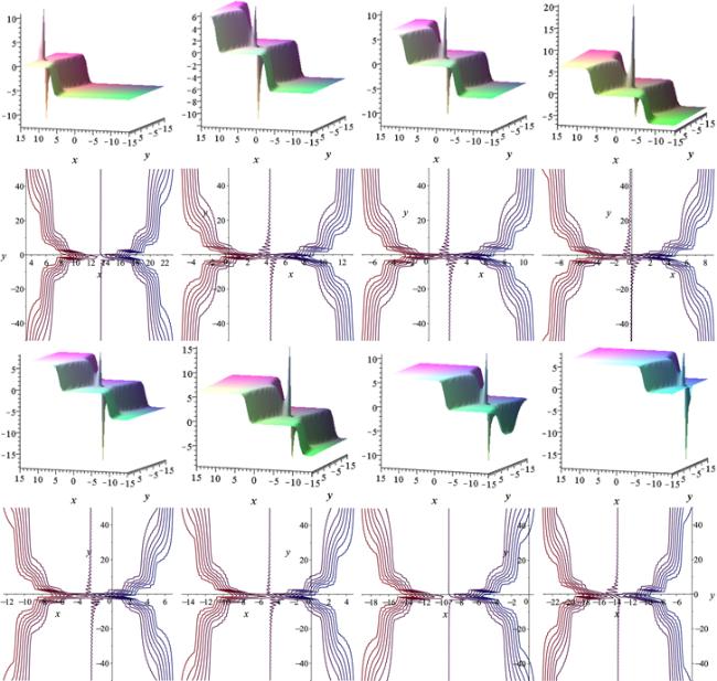
We choose the following parameters to illustrate the interaction solution (54) between the high-order lump-type solution and the three-wave solutions to the (3+1)-dimensional Jimbo–Miwa equation (1),
The physical properties and structures for interaction solution (54) are shown in figure 1. It shows the three-dimensional dynamic graphs and contour plots in the (x, y)-plane when $t=-60,-20,-10,0,10,20,40,60$ respectively. The three-dimensional graphs reflect the localized structures. We can see that the high-order lump-type wave, double exponential function, trigonometric function and hyperbolic function waves react with each other and keep moving forward.
Figure 1. Three-dimensional plots and contour plots of the wave with the parameters (55) at times t = − 60, − 20, − 10,0,10,20,40,60.
The wave consists of two parts, including a high-order lump-type wave and an other functions wave (double-exponential function, trigonometric function and hyperbolic function). The lump wave moves in one direction to the other with the variable t. The amplitude of the lump changes with the variable t, and especially when t = 0, the energy and amplitude of the lump–soliton reaches the maximum. This phenomenon is very strange and analogous to rogue waves. The process of interaction changes the amplitudes, shapes and velocities of both waves. This type of interaction solutions provide a method to forecast the appearance of rogue waves, such as financial rogue waves, optical rogue waves and plasma rogue waves, through analyzing the relations between the lump wave part and the soliton wave part.
4.2. Three-dimensional, contour and density plots of the interaction solutions to Case 4.1
If we substitute the coefficient of Case 4.1 into (12), we can get f2 as follows:
where ${a}_{0},{a}_{12},{a}_{20},{a}_{23},{a}_{30},{a}_{31},{a}_{34},{b}_{30},{b}_{32},{b}_{40},{b}_{42}({m}_{1}{a}_{31}{a}_{34}\,\ne 0)$ are arbitrary real constants. By substituting (56) into (2), we get interaction solution (54) to (3+1)-dimensional Jimbo–Miwa Equation (1).
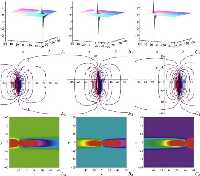
We choose the following parameters to illustrate the interaction solution (54) between the high-order lump-type solution and the cos–cosh solitary wave solutions of the (3+1)-dimensional Jimbo–Miwa equation (1),
The physical properties and structures of the interaction solution (54) are shown in figure 2. It shows the three-dimensional dynamic graphs A1, B1, C1, corresponding contour maps A2, B2, C2 and density plots A3, B3, C3 in the (x, y)-plane when t = − 20, 0, 20, respectively. The three-dimensional graphs reflect the localized structures, and the density plots show the energy distribution. We can see that the high-order lump-type wave, trigonometric function and hyperbolic function wave react with each other and keep moving forward.
Figure 2. Three-dimensional plots, contour plots and density plots of the wave with the parameters (57) at times t = − 20 (A1,A2,A3), t = 0 (B1,B2,B3), t = 20 (C1,C2,C3).
5. Conclusion
In this paper, we gave the form of general interaction solution to the (3+1)-dimensional Jimbo–Miwa equation. The general interaction solution contained classical interaction solutions, such as the lump–kink solution and the lump–soliton solution. As an example, by using the generalized bilinear method and symbolic computation software Maple, we successfully construct novel interaction solutions between the high-order lump-type solution and other functions of the (3+1)-dimensional Jimbo–Miwa equation, such as, three-wave solutions, breather solutions, solitary wave solutions, cos–cosh solitary wave solutions, lump–soliton solutions and cos periodic wave solutions. Three-dimensional plots, contour plots and density plots of these waves may be observed in figures 1–2, respectively. We can find the physical structure and characteristics of the interactions between high-order lump-type solutions and other function waves.
The new interaction solutions obtained in this paper will greatly expand the exact solutions to the (3+1)-dimensional Jimbo–Miwa equation in the existing literature [3–6, 12, 13, 24–30, 51–54]. These results are significant to understand the propagation processes of nonlinear waves in fluid mechanics and the explanation of some special physical problems.
Conflict of Interest
The authors declare that they have no conflicts of interest.


