Welcome to visit Communications in Theoretical Physics,
Mathematical Physics

A (2+1)-dimensional nonlinear model for Rossby waves in stratified fluids and its solitary solution

  • Li-Guo Chen(陈利国) 1, 2 ,
  • Lian-Gui Yang(杨联贵) , 1 ,
  • Rui-Gang Zhang(张瑞岗) 1 ,
  • Quan-Sheng Liu(刘全生) 1 ,
  • Ji-Feng Cui(崔继峰) 3
Expand
  • 1School of Mathematical Sciences, Inner Mongolia University, Hohhot 010021, China
  • 2School of Statistics and Mathematics, Inner Mongolia University of Finance and Economics, Hohhot 010070, China
  • 3College of Science, Inner Mongolia University of Technology, Hohhot 010051, China

Received date: 2019-11-27

  Revised date: 2020-02-10

  Accepted date: 2020-02-11

  Online published: 2020-04-08

Copyright

© 2020 Chinese Physical Society and IOP Publishing Ltd

Abstract

In this paper, we investigate a (2+1)-dimensional nonlinear equation model for Rossby waves in stratified fluids. We derive a forced Zakharov–Kuznetsov(ZK)–Burgers equation from the quasi-geostrophic potential vorticity equation with dissipation and topography under the generalized beta effect, and by utilizing temporal and spatial multiple scale transform and the perturbation expansion method. Through the analysis of this model, it is found that the generalized beta effect and basic topography can induce nonlinear waves, and slowly varying topography is an external impact factor for Rossby waves. Additionally, the conservation laws for the mass and energy of solitary waves are analyzed. Eventually, the solitary wave solutions of the forced ZK–Burgers equation are obtained by the simplest equation method as well as the new modified ansatz method. Based on the solitary wave solutions obtained, we discuss the effects of dissipation and slowly varying topography on Rossby solitary waves.

Cite this article

Li-Guo Chen(陈利国) , Lian-Gui Yang(杨联贵) , Rui-Gang Zhang(张瑞岗) , Quan-Sheng Liu(刘全生) , Ji-Feng Cui(崔继峰) . A (2+1)-dimensional nonlinear model for Rossby waves in stratified fluids and its solitary solution[J]. Communications in Theoretical Physics, 2020 , 72(4) : 045004 . DOI: 10.1088/1572-9494/ab7703

1. Introduction

Solitary waves were discovered by Russell [1]. These waves exist as a natural phenomenon due to the balance between dispersion and nonlinearity. Several kinds of nonlinear equation models were used to characterize the evolution of waves such as acoustic waves, gravity-inertial waves and Rossby waves. The nonlinear wave model, especially on a solitary wave, is also of great significance in other fields [24]. Solitary waves are one of the wave phenomena with the most theoretical significance and research value. The Korteweg–de Vries (KdV) equation is the classical equation model used to describe solitary waves [5], and its classical solitary wave solution has been presented [610].
In the complex atmospheric and oceanic wave motions, Rossby waves are extremely important large-scale waves, caused by the rotation of the Earth. Many kinds of nonlinear equation models were generated and applied to characterize the evolution of a Rossby wave’s amplitude and to explain some further weather phenomena. Many studies prove that Rossby waves affect the weather and climate change on a planet, such as the red spot in the atmosphere of Jupiter, atmospheric blocking and the Southern Oscillation [1113]. Thus, the research on Rossby solitary waves can provide a theoretical basis for actual weather and ocean forecasting. Historically, theories on nonlinear large-scale Rossby waves are significant research subjects. Different types of the nonlinear KdV equation were derived to reveal some physical mechanisms of Rossby waves in the past [1424], In recent years, through Gardner–Morikawa transform and the perturbation expansion method, the nonlinear equation models for describing the formation of Rossby waves or envelope waves have been derived under the traditional beta plane approximation [2534], However, the beta is not constant for actual atmospheric motions. In barotropic fluids, Liu et al [35] studied the generation of Rossby waves under a change in the beta plane. Song et al [36, 37] generalized the above results to a general case, and concluded that the generalized beta effect can induce solitary Rossby waves. Li et al [38] obtained the evolution of the Rossby wave envelope with the generalized beta effect in stratified fluids.
High-dimensional nonlinear equation models can be more accurate for describing the propagation of Rossby waves in the real atmosphere and ocean. Over the last few years, plenty of studies have applied higher-dimensional nonlinear equations to explore the formation of Rossby waves in barotropic fluids. Gottwald derived the Zakharov–Kuznetsov (ZK) equation [39]. Yang et al [40] obtained the three-dimensional ZK–Burgers equation. Zhao et al [41] derived the ZK-mZK equation, and considered the impact of a complete Coriolis force on Rossby waves. Zhang et al [42, 43] obtained the (2+1)-dimensional generalized forced ZK equation and ZK equation. Liu et al [44] derived a new (2+1)-dimensional generalized Boussinesq equation. Chen et al [45] derived a new generalized (2+1)-dimensional nonlinear mKdV–Burgers equation, and analyzed the effects of generalized beta, shear basic flow and dissipation on the evolution of solitary waves. It is known that a stratified fluid is more appropriate for actual atmospheric and oceanic motions. However, due to density stratification and other impact factors, it is hard to obtain models for Rossby waves in stratified fluids. Lu et al [46] derived the classical (1+1)-dimensional Boussinesq equation in stratified fluids. Meng et al [47] obtained the (1+1)-dimensional mKdV equation to describe Rossby waves. Therefore, it is essential to study the high-dimensional models for Rossby waves in stratified fluid to better explain the nonlinear dynamics of Rossby waves. Dissipation and topography are extremely important factors in large-scale motion. In particular, the impacts of varying topography on Rossby solitary waves have attracted the attention of many scholars [4851]. However, the effect of varying topography on Rossby solitary waves in stratified fluids has not been examined. Ren et al [52] studied (3+1)-dimensional Rossby waves in cylindrical coordinates using the Lie symmetry approach. Recently, plenty of studies have applied fractional order model equations to describe the formation process of Rossby waves in the atmosphere and ocean [5360].
In the present study, we obtain a ZK–Burgers equation with dissipation and topography forcing to describe Rossby waves in stratified fluids. The rest of the paper is organized as follows: in section 2, using temporal and spatial transform and a perturbation expansion method, a new forced (2+1)-dimensional nonlinear ZK–Burgers equation is derived. In addition, we discuss the important physical factors that induce the nonlinear Rossby waves, and analyze the conservation laws of solitary waves. In section 3, the single solitary wave solutions of the ZK equation are obtained using the simplest equation method. The asymptotic solitary wave solutions of the ZK–Burgers equation under dissipation and topographic forcing are obtained by employing a new modified ansatz method. We discuss the effects of dissipation and slowly varying topography on solitary waves. Conclusions are presented in section 4.

2. Model and method

2.1. Derivation of the forced ZK–Burgers equation model

The dimensionless geostrophic potential vorticity equation, including topography, h(x, y, t) and a heating source, Q(y, z), is as follows [38, 47, 61]:
$\begin{eqnarray}\begin{array}{l}\left(\displaystyle \frac{\partial }{\partial t}+\displaystyle \frac{\partial \psi }{\partial x}\displaystyle \frac{\partial }{\partial y}-\displaystyle \frac{\partial \psi }{\partial y}\displaystyle \frac{\partial }{\partial x}\right)\left[{{\rm{\nabla }}}^{2}\psi +\beta (y)y\right.\\ \qquad \left.+\,\displaystyle \frac{f}{{\rho }_{s}}\displaystyle \frac{\partial }{\partial z}\left(\displaystyle \frac{{\rho }_{s}}{s}\displaystyle \frac{\partial \psi }{\partial z}\right)\right]=\displaystyle \frac{f}{{\rho }_{s}}\displaystyle \frac{\partial }{\partial z}\left(\displaystyle \frac{{\rho }_{s}}{s}Q\right),\end{array}\end{eqnarray}$
where ψ is the geostrophic stream function, f is the Coriolis parameter, β(y) is the generalized Rossby parameter [36], $s=\tfrac{{N}^{2}}{f}$ and ρs are functions of only z, N is the Brünt–Vaisala frequency, ρs is the stratified density and ∇2 denotes the two-dimensional Laplace operator.
The lateral boundary conditions are
$\begin{eqnarray}\displaystyle \frac{\partial \psi }{\partial x}=0,y=0,1.\end{eqnarray}$
The upper boundary condition is
$\begin{eqnarray}{\rho }_{s}\psi \to 0,z\to \infty .\end{eqnarray}$
The lower boundary condition, the governing equation, including heat, turbulent dissipation and topography, is
$\begin{eqnarray}\begin{array}{l}\left(\displaystyle \frac{\partial }{\partial t}+\displaystyle \frac{\partial \psi }{\partial x}\displaystyle \frac{\partial }{\partial y}-\displaystyle \frac{\partial \psi }{\partial y}\displaystyle \frac{\partial }{\partial x}\right)\displaystyle \frac{\partial \psi }{\partial z}\\ \quad +\,s\left(\displaystyle \frac{\partial \psi }{\partial x}\displaystyle \frac{\partial h}{\partial y}-\displaystyle \frac{\partial \psi }{\partial y}\displaystyle \frac{\partial h}{\partial x}\right)+{\left|\displaystyle \frac{k}{2f}\right|}^{\tfrac{1}{2}}s{{\rm{\nabla }}}^{2}\psi =Q,z=0,\end{array}\end{eqnarray}$
where k is the dissipative coefficient.
We assume the total stream function is
$\begin{eqnarray}\psi (x,y,z,t)=-{\int }_{0}^{y}[\overline{u}(y,z)-{c}_{0}]{\rm{d}}y+\epsilon \psi ^{\prime} (x,y,z,t),\end{eqnarray}$
where $\overline{u}(y,z)$ is the basic shear flow function, c0 is the velocity of the linear wave, ϵ ≪ 1 is a small parameter and $\psi ^{\prime} $ is the disturbed stream function.
To balance between topography and nonlinearity, we assume the topography as follows:
$\begin{eqnarray}h(x,y,t)={h}_{0}(y)+{\epsilon }^{2}{h}_{1}(x,t),\end{eqnarray}$
where h0(y) represents the basic topographic function, and h1(x, t) represents the slowly varying topography function. Substituting equations (5) and (6) into equations (1)–(4) we obtain
$\begin{eqnarray}\begin{array}{l}\left[\displaystyle \frac{\partial }{\partial t}+(\overline{u}-{c}_{0})\displaystyle \frac{\partial }{\partial x}+\epsilon \left(\displaystyle \frac{\partial \psi ^{\prime} }{\partial x}\displaystyle \frac{\partial }{\partial y}-\displaystyle \frac{\partial \psi ^{\prime} }{\partial y}\displaystyle \frac{\partial }{\partial x}\right)\right]\\ \quad \times \,\left[{{\rm{\nabla }}}^{2}\psi ^{\prime} +\displaystyle \frac{f}{{\rho }_{s}}\displaystyle \frac{\partial }{\partial z}\left(\displaystyle \frac{{\rho }_{s}}{s}\displaystyle \frac{\partial \psi ^{\prime} }{\partial z}\right)\right]+p(y,z)\displaystyle \frac{\partial \psi ^{\prime} }{\partial x}=0,\end{array}\end{eqnarray}$
$\begin{eqnarray}\begin{array}{l}\left[\displaystyle \frac{\partial }{\partial t}+(\overline{u}-{c}_{0})\displaystyle \frac{\partial }{\partial x}+\epsilon \left(\displaystyle \frac{\partial \psi ^{\prime} }{\partial x}\displaystyle \frac{\partial }{\partial y}-\displaystyle \frac{\partial \psi ^{\prime} }{\partial y}\displaystyle \frac{\partial }{\partial x}\right)\right]\displaystyle \frac{\partial \psi ^{\prime} }{\partial z}\\ -\,\displaystyle \frac{\partial \psi ^{\prime} }{\partial x}\displaystyle \frac{\partial \overline{u}}{\partial z}+{{sh}}_{0}^{{\prime} }(y)\displaystyle \frac{\partial \psi ^{\prime} }{\partial x}\\ +\,\epsilon s\left[(\overline{u}-{c}_{0})-\epsilon \displaystyle \frac{\partial \psi ^{\prime} }{\partial y}\right]\displaystyle \frac{\partial {h}_{1}}{\partial x}+{\epsilon }^{2}\lambda s{{\rm{\nabla }}}^{2}\psi ^{\prime} =0,z\,=\,0,\end{array}\end{eqnarray}$
$\begin{eqnarray}\displaystyle \frac{\partial \psi ^{\prime} }{\partial x}=0,y=0,1,\end{eqnarray}$
$\begin{eqnarray}{\rho }_{s}\psi ^{\prime} \to 0,z\to \infty ,\end{eqnarray}$
where $p(y,z)=\left[\tfrac{\partial }{\partial y}(\beta (y)y)-\tfrac{{\partial }^{2}\overline{u}}{\partial {y}^{2}}-\tfrac{f}{{\rho }_{s}}\tfrac{\partial }{\partial z}\left(\tfrac{{\rho }_{s}}{s}\tfrac{\partial \overline{u}}{\partial z}\right)\right]$. To balance the external heating source, the diffusion of shearing flow $\overline{u}$, turbulent dissipation and nonlinearity, we assume
$\begin{eqnarray}{\left|\displaystyle \frac{k}{2f}\right|}^{\tfrac{1}{2}}={\epsilon }^{2}\lambda ,\end{eqnarray}$
$\begin{eqnarray}\displaystyle \frac{\partial }{\partial z}\left(\displaystyle \frac{{\rho }_{s}}{s}Q\right)=0,\end{eqnarray}$
$\begin{eqnarray}{\left|\displaystyle \frac{k}{2f}\right|}^{\tfrac{1}{2}}s\left(\displaystyle \frac{\partial \overline{u}}{\partial y}\right)+Q=0,z=0.\end{eqnarray}$
Based on the temporal and spatial multiple scales feature of the motions of large-scale waves, we adopt the following transform:
$\begin{eqnarray}X=\epsilon x,\ Y=\epsilon y,\ T={\epsilon }^{3}t,\ z=z.\end{eqnarray}$
and assume
$\begin{eqnarray}{h}_{1}(x,t)={\epsilon }^{2}H(X,T).\end{eqnarray}$
The disturbed stream function $\psi ^{\prime} $ is expanded as follows:
$\begin{eqnarray}\psi ^{\prime} (X,y,Y,T)=\epsilon {\psi }_{0}+{\epsilon }^{2}{\psi }_{1}+{\epsilon }^{3}{\psi }_{2}+\cdots .\end{eqnarray}$
Substituting equations (14)–(16) into equations (7)–(10) yields
$\begin{eqnarray}O({\epsilon }^{1}):\left\{\begin{array}{l}(\overline{u}-{c}_{0})\tfrac{\partial }{\partial X}\left[\tfrac{{\partial }^{2}{\psi }_{0}}{\partial {y}^{2}}+\tfrac{f}{{\rho }_{s}}\tfrac{\partial }{\partial z}\left(\tfrac{{\rho }_{s}}{s}\tfrac{\partial {\psi }_{0}}{\partial z}\right)\right]+p(y,z)\tfrac{\partial {\psi }_{0}}{\partial X}\\ =\ 0,\\ (\overline{u}-{c}_{0})\tfrac{\partial }{\partial X}\left(\tfrac{\partial {\psi }_{0}}{\partial z}\right)-\tfrac{\partial {\psi }_{0}}{\partial X}\tfrac{\partial \overline{u}}{\partial z}+{{sh}}_{0}^{{\prime} }(y)\tfrac{\partial {\psi }_{0}}{\partial X}=0,\\ z=0,\\ \tfrac{\partial {\psi }_{0}}{\partial x}=0,y=0,1,\\ {\rho }_{s}{\psi }_{0}\to 0,z\to \infty ,\end{array}\right.\end{eqnarray}$
$\begin{eqnarray}O({\epsilon }^{2}):\left\{\begin{array}{l}(\overline{u}-{c}_{0})\tfrac{\partial }{\partial X}\left[\tfrac{{\partial }^{2}{\psi }_{1}}{\partial {y}^{2}}+\tfrac{f}{{\rho }_{s}}\tfrac{\partial }{\partial z}\left(\tfrac{{\rho }_{s}}{s}\tfrac{\partial {\psi }_{1}}{\partial z}\right)\right]+p(y,z)\\ \tfrac{\partial {\psi }_{1}}{\partial X}=0,\\ (\overline{u}-{c}_{0})\tfrac{\partial }{\partial X}\left(\tfrac{\partial {\psi }_{1}}{\partial z}\right)-\tfrac{\partial {\psi }_{1}}{\partial X}\tfrac{\partial \overline{u}}{\partial z}+{{sh}}_{0}^{{\prime} }(y)\tfrac{\partial {\psi }_{1}}{\partial X}=0,\\ z=0,\\ \tfrac{\partial {\psi }_{1}}{\partial x}=0,y=0,1,\\ {\rho }_{s}{\psi }_{1}\to 0,z\to \infty ,\end{array}\right.\end{eqnarray}$
$\begin{eqnarray}O({\epsilon }^{3}):\left\{\begin{array}{l}(\overline{u}-{c}_{0})\tfrac{\partial }{\partial X}\left[\tfrac{{\partial }^{2}{\psi }_{2}}{\partial {y}^{2}}+\tfrac{f}{{\rho }_{s}}\tfrac{\partial }{\partial z}\left(\tfrac{{\rho }_{s}}{s}\tfrac{\partial {\psi }_{2}}{\partial z}\right)\right]+p(y,z)\\ \tfrac{\partial {\psi }_{2}}{\partial X}=-F,\\ (\overline{u}-{c}_{0})\tfrac{\partial }{\partial X}\left(\tfrac{\partial {\psi }_{2}}{\partial z}\right)-\tfrac{\partial {\psi }_{2}}{\partial X}\tfrac{\partial \overline{u}}{\partial z}+{{sh}}_{0}^{{\prime} }(y)\tfrac{\partial {\psi }_{2}}{\partial X}=-D,\\ z=0,\\ \tfrac{\partial {\psi }_{2}}{\partial x}=0,y=0,1,\\ {\rho }_{s}{\psi }_{2}\to 0,z\to \infty ,\end{array}\right.\end{eqnarray}$
where
$\begin{eqnarray}\begin{array}{rcl}F & = & \left[\displaystyle \frac{\partial }{\partial T}+\left(\displaystyle \frac{\partial {\psi }_{0}}{\partial X}\displaystyle \frac{\partial }{\partial y}-\displaystyle \frac{\partial {\psi }_{0}}{\partial y}\displaystyle \frac{\partial }{\partial X}\right)\right]\\ & & \times \left[\displaystyle \frac{{\partial }^{2}{\psi }_{0}}{\partial {y}^{2}}+\displaystyle \frac{f}{{\rho }_{s}}\displaystyle \frac{\partial }{\partial z}\left(\displaystyle \frac{{\rho }_{s}}{s}\displaystyle \frac{\partial {\psi }_{0}}{\partial z}\right)\right]\\ & & +2(\overline{u}-{c}_{0})\displaystyle \frac{\partial }{\partial X}\left(\displaystyle \frac{{\partial }^{2}{\psi }_{1}}{\partial y\partial Y}\right)\\ & & +(\overline{u}-{c}_{0})\displaystyle \frac{\partial }{\partial X}\left(\displaystyle \frac{{\partial }^{2}{\psi }_{0}}{\partial {X}^{2}}+\displaystyle \frac{{\partial }^{2}{\psi }_{0}}{\partial {Y}^{2}}\right),\end{array}\end{eqnarray}$
$\begin{eqnarray}\begin{array}{rcl}D & = & \displaystyle \frac{\partial }{\partial T}\left(\displaystyle \frac{\partial {\psi }_{0}}{\partial z}\right)+\left(\displaystyle \frac{\partial {\psi }_{0}}{\partial X}\displaystyle \frac{\partial }{\partial y}-\displaystyle \frac{\partial {\psi }_{0}}{\partial y}\displaystyle \frac{\partial }{\partial X}\right)\displaystyle \frac{\partial {\psi }_{0}}{\partial z}\\ & & +s(\overline{u}-{c}_{0})\displaystyle \frac{\partial H}{\partial X}+\lambda s\displaystyle \frac{{\partial }^{2}{\psi }_{0}}{\partial {Y}^{2}},z\,=\,0.\end{array}\end{eqnarray}$
Using the method of separating variables, we assume that ψ0 and ψ1 are the following forms, respectively,
$\begin{eqnarray}{\psi }_{0}=A(X,Y,T){\phi }_{0}(y,z).\end{eqnarray}$
and
$\begin{eqnarray}{\psi }_{1}=\displaystyle \frac{\partial }{\partial Y}A(X,Y,T){\phi }_{1}(y,z).\end{eqnarray}$
Substituting equations (22) and (23) into equations (17) and (18), respectively, we obtain
$\begin{eqnarray}\left\{\begin{array}{l}(\overline{u}-{c}_{0})\left[\tfrac{{\partial }^{2}}{\partial {y}^{2}}+\tfrac{f}{{\rho }_{s}}\tfrac{\partial }{\partial z}\left(\tfrac{{\rho }_{s}}{s}\tfrac{\partial }{\partial z}\right)\right]{\phi }_{0}+p(y,z){\phi }_{0}=0,\\ (\overline{u}-{c}_{0})\tfrac{\partial {\phi }_{0}}{\partial z}-\left[\tfrac{\partial \overline{u}}{\partial z}-{{sh}}_{0}^{{\prime} }(y)\right]{\phi }_{0},z=0,\\ {\phi }_{0}(y,z)=0,y=0,1,\\ {\rho }_{s}{\phi }_{0}\to 0,z\to \infty .\end{array}\right.\end{eqnarray}$
and
$\begin{eqnarray}\left\{\begin{array}{l}(\overline{u}-{c}_{0})\left[\tfrac{{\partial }^{2}}{\partial {y}^{2}}+\tfrac{f}{{\rho }_{s}}\tfrac{\partial }{\partial z}\left(\tfrac{{\rho }_{s}}{s}\tfrac{\partial }{\partial z}\right)\right]{\phi }_{1}+p(y,z){\phi }_{1}\\ =-2(\overline{u}-{c}_{0})\tfrac{\partial {\phi }_{0}}{\partial y},\\ (\overline{u}-{c}_{0})\tfrac{\partial {\phi }_{1}}{\partial z}-\left[\tfrac{\partial \overline{u}}{\partial z}-{{sh}}_{0}^{{\prime} }(y)\right]{\phi }_{1},z=0,\\ {\phi }_{1}(y,z)=0,y=0,1,\\ {\rho }_{s}{\phi }_{1}\to 0,z\to \infty .\end{array}\right.\end{eqnarray}$
In equation (19), the first equation multiplied by $\tfrac{{\rho }_{s}{\phi }_{0}}{\overline{u}-{c}_{0}}$, yields
$\begin{eqnarray}\begin{array}{l}\displaystyle \frac{\partial }{\partial y}{\rho }_{s}\left[{\phi }_{0}\displaystyle \frac{\partial }{\partial y}\left(\displaystyle \frac{\partial {\psi }_{2}}{\partial X}\right)-\displaystyle \frac{\partial {\psi }_{2}}{\partial X}\displaystyle \frac{\partial {\phi }_{0}}{\partial y}\right]\\ \quad +\,f\displaystyle \frac{\partial }{\partial z}\displaystyle \frac{{\rho }_{s}}{s}\left[{\phi }_{0}\displaystyle \frac{\partial }{\partial z}\left(\displaystyle \frac{\partial {\psi }_{2}}{\partial X}\right)-\displaystyle \frac{\partial {\psi }_{2}}{\partial X}\displaystyle \frac{\partial {\phi }_{0}}{\partial z}\right]\\ \ =\,\displaystyle \frac{\partial A}{\partial T}\displaystyle \frac{{\rho }_{s}{\phi }_{0}^{2}p(y,z)}{{\left(\overline{u}-{c}_{0}\right)}^{2}}+A\displaystyle \frac{\partial A}{\partial X}\displaystyle \frac{{\rho }_{s}{\phi }_{0}^{3}}{\overline{u}-{c}_{0}}\displaystyle \frac{\partial }{\partial y}\left(\displaystyle \frac{p(y,z)}{\overline{u}-{c}_{0}}\right)\\ \quad -\,\displaystyle \frac{{\partial }^{3}A}{\partial X\partial {Y}^{2}}{\rho }_{s}\left({\phi }_{0}^{2}+2{\phi }_{0}\displaystyle \frac{\partial {\phi }_{1}}{\partial y}\right)+\displaystyle \frac{{\partial }^{3}A}{\partial {X}^{3}}(-{\rho }_{s}{\phi }_{0}^{2}).\end{array}\end{eqnarray}$
And the second equation multiplied by $\tfrac{f{\rho }_{s}{\phi }_{0}}{s(\overline{u}-{c}_{0})}$, yields
$\begin{eqnarray}\begin{array}{l}\displaystyle \frac{f{\rho }_{s}{\phi }_{0}}{s}\displaystyle \frac{\partial }{\partial z}\left(\displaystyle \frac{\partial {\psi }_{2}}{\partial X}\right)-\displaystyle \frac{1}{\overline{u}-{c}_{0}}\left[\displaystyle \frac{\partial \overline{u}}{\partial z}-{{sh}}_{0}^{{\prime} }(y)\right]\displaystyle \frac{\partial {\psi }_{2}}{\partial X}\\ \quad =\,-\displaystyle \frac{\partial A}{\partial T}\displaystyle \frac{f{\phi }_{0}}{\overline{u}-{c}_{0}}\displaystyle \frac{{\rho }_{s}}{s}\displaystyle \frac{\partial {\phi }_{0}}{\partial z}-A\displaystyle \frac{\partial A}{\partial X}\displaystyle \frac{f}{\overline{u}-{c}_{0}}\displaystyle \frac{{\rho }_{s}}{s}\left({\phi }_{0}^{2}\displaystyle \frac{{\partial }^{2}{\phi }_{0}}{\partial y\partial z}\right)\\ \qquad -\,f{\rho }_{s}{\phi }_{0}\displaystyle \frac{\partial H}{\partial X}+\lambda A\displaystyle \frac{f{\rho }_{s}{\phi }_{0}}{\overline{u}-{c}_{0}}\displaystyle \frac{{\partial }^{2}{\phi }_{0}}{\partial {y}^{2}},z\,=\,0,\end{array}\end{eqnarray}$
where $\overline{u}-{c}_{0}\ne 0$. Equation (26) is integrated from 0 to 1 for variable y, and from 0 to $\infty $ for variable z. Equation (27) is integrated from 0 to 1 for variable y. Finally, using boundary conditions of equations (24) and (25) we obtain
$\begin{eqnarray}\displaystyle \frac{\partial A}{\partial T}+{\alpha }_{1}A\displaystyle \frac{\partial A}{\partial X}+{\alpha }_{2}\displaystyle \frac{{\partial }^{3}A}{\partial {X}^{3}}+{\alpha }_{3}\displaystyle \frac{{\partial }^{3}A}{\partial X\partial {Y}^{2}}+\eta A=\gamma \displaystyle \frac{\partial H}{\partial X},\end{eqnarray}$
where
$\begin{eqnarray}\left\{\begin{array}{l}{\alpha }_{1}=\tfrac{1}{\sigma }{\displaystyle \int }_{0}^{\infty }{\displaystyle \int }_{0}^{1}\tfrac{{\rho }_{s}{\phi }_{0}^{3}}{\overline{u}-{c}_{0}}\tfrac{\partial }{\partial y}\left(\tfrac{p(y,z)}{\overline{u}-{c}_{0}}\right){\rm{d}}y{\rm{d}}z\\ -\tfrac{1}{\sigma }{\displaystyle \int }_{0}^{1}{\left[\tfrac{f}{\overline{u}-{c}_{0}}\tfrac{{\rho }_{s}}{s}\left({\phi }_{0}^{2}\tfrac{{\partial }^{2}{\phi }_{0}}{\partial y\partial z}-{\phi }_{0}\tfrac{\partial {\phi }_{0}}{\partial y}\tfrac{\partial {\phi }_{0}}{\partial z}\right)\right]}_{z=0}{\rm{d}}y,\\ {\alpha }_{2}=-\tfrac{1}{\sigma }{\displaystyle \int }_{0}^{\infty }{\displaystyle \int }_{0}^{1}{\rho }_{s}{\phi }_{0}^{2}{\rm{d}}y{\rm{d}}z,\\ {\alpha }_{3}=-\tfrac{1}{\sigma }{\displaystyle \int }_{0}^{\infty }{\displaystyle \int }_{0}^{1}{\rho }_{s}\left({\phi }_{0}^{2}+2{\phi }_{0}\tfrac{\partial {\phi }_{1}}{\partial y}\right){\rm{d}}y{\rm{d}}z,\\ \eta =\tfrac{\lambda }{\sigma }{\displaystyle \int }_{0}^{1}{\left[\tfrac{f{\rho }_{s}{\phi }_{0}}{\overline{u}-{c}_{0}}\tfrac{{\partial }^{2}{\phi }_{0}}{\partial {y}^{2}}\right]}_{z=0}{\rm{d}}y,\\ \gamma =\tfrac{f}{\sigma }{\displaystyle \int }_{0}^{1}{\left[{\rho }_{s}{\phi }_{0}\right]}_{z=0}{\rm{d}}y,\\ \sigma ={\displaystyle \int }_{0}^{\infty }{\displaystyle \int }_{0}^{1}\tfrac{{\rho }_{s}{\phi }_{0}^{2}p(y,z)}{{\left(\overline{u}-{c}_{0}\right)}^{2}}{\rm{d}}y{\rm{d}}z-{\displaystyle \int }_{0}^{1}{\left[\tfrac{f{\phi }_{0}}{\overline{u}-{c}_{0}}\tfrac{{\rho }_{s}}{s}\tfrac{\partial {\phi }_{0}}{\partial z}\right]}_{z=0}{\rm{d}}y.\end{array}\right.\end{eqnarray}$

φ0 and φ1 are determined by eigen equations (24) and (25). Equation (28) is the new forced (2+1)-dimensional nonlinear equation for describing the evolution of Rossby waves in stratified fluids. The new model is different to [40, 42, 43]. The term with coefficient α1 indicates the effects of multiple physical factors on the formation of nonlinear Rossby waves; that is, the generalized β(y), stratification s, and the shear flow $\overline{u}$, basic topography h0(y). From the eigen equations (24), it is found that ${\alpha }_{1}\ne 0$ when $\overline{u}=0,{\rho }_{s}$ and s are constants, respectively; this shows that the generalized beta and basic topography are all essential factors for the formation of solitary waves. The term with coefficient α2 and α3 represents the dispersion relation for linear Rossby waves, which is related to the generalized beta and the shear basic flow and stratification. Here, η A represents the dissipation term, while $\gamma \tfrac{\partial H}{\partial X}$ represents the external force factor, caused by slowly varying topography. The above theoretical analysis shows that the dynamics of Rossby waves are very complex in real atmospheric and oceanic motion. On the other hand, when α3 = 0 equation (28) reduces to the case considered by Jiang et al [24]. When η = 0 and γ = 0, equation (28) is the normal ZK equation. Thus, equation (28) is the generalization of previous research results for stratified fluids, and is called the forced (2+1)-dimensional ZK–Burgers equation.

2.2. Analysis of Rossby solitary wave conservation law

In equation (28), we only consider the condition of η > 0. We do not consider η < 0, because of the instability of disturbance. To analyze the conservation law of Rossby waves, we may assume that
$\begin{eqnarray}\left(A,\displaystyle \frac{\partial A}{\partial X},\displaystyle \frac{\partial A}{\partial Y},\displaystyle \frac{{\partial }^{2}A}{\partial {X}^{2}},\displaystyle \frac{{\partial }^{2}A}{\partial {Y}^{2}},\displaystyle \frac{{\partial }^{2}A}{\partial X\partial Y}\right)\to 0\ {as}\ | X| ,| Y| \to 0.\end{eqnarray}$
Equation (28) is transformed into as follows:
$\begin{eqnarray}\displaystyle \frac{\partial }{\partial T}A+\displaystyle \frac{\partial }{\partial X}\left(\displaystyle \frac{{\alpha }_{1}}{2}{A}^{2}+{\alpha }_{2}\displaystyle \frac{{\partial }^{2}A}{\partial {X}^{2}}+{\alpha }_{3}\displaystyle \frac{{\partial }^{2}A}{\partial {Y}^{2}}\right)+\eta A=\gamma \displaystyle \frac{\partial H}{\partial X}.\end{eqnarray}$
Equation (31) is integrated with X and Y, and the mass equation for solitary waves is obtained
$\begin{eqnarray}\begin{array}{l}\displaystyle \frac{\partial }{\partial T}{\displaystyle \int }_{-\infty }^{+\infty }{\displaystyle \int }_{-\infty }^{+\infty }A{\rm{d}}X{\rm{d}}Y+\eta {\displaystyle \int }_{-\infty }^{+\infty }{\displaystyle \int }_{-\infty }^{+\infty }A{\rm{d}}X{\rm{d}}Y\\ \quad =\,\gamma {\displaystyle \int }_{-\infty }^{+\infty }{\displaystyle \int }_{-\infty }^{+\infty }\displaystyle \frac{\partial H}{\partial X}{\rm{d}}X{\rm{d}}Y.\end{array}\end{eqnarray}$
Equation (28) multiplied by $2A$ yields:
$\begin{eqnarray}\begin{array}{l}\displaystyle \frac{\partial }{\partial T}{A}^{2}+\displaystyle \frac{\partial }{\partial X}\left[\displaystyle \frac{2{\alpha }_{1}}{3}{A}^{3}+2{\alpha }_{2}A\displaystyle \frac{{\partial }^{2}A}{\partial {X}^{2}}-{\alpha }_{2}{\left(\displaystyle \frac{\partial A}{\partial X}\right)}^{2}\right.\\ -\left.{\alpha }_{3}{\left(\displaystyle \frac{\partial A}{\partial Y}\right)}^{2}\right]\\ +\,{\alpha }_{3}\displaystyle \frac{\partial }{\partial Y}\left(A\displaystyle \frac{{\partial }^{2}A}{\partial X\partial Y}\right)+2\eta {A}^{2}=2\gamma A\displaystyle \frac{\partial H}{\partial X}.\end{array}\end{eqnarray}$
Equation (33) is integrated with X and Y, and the energy equation for solitary waves is obtained
$\begin{eqnarray}\begin{array}{l}\displaystyle \frac{\partial }{\partial T}{\displaystyle \int }_{-\infty }^{+\infty }{\displaystyle \int }_{-\infty }^{+\infty }{A}^{2}{\rm{d}}X{\rm{d}}Y+2\eta {\displaystyle \int }_{-\infty }^{+\infty }{\displaystyle \int }_{-\infty }^{+\infty }{A}^{2}{\rm{d}}X{\rm{d}}Y\\ \quad =\,2\gamma {\displaystyle \int }_{-\infty }^{+\infty }{\displaystyle \int }_{-\infty }^{+\infty }A\displaystyle \frac{\partial H}{\partial X}{\rm{d}}X{\rm{d}}Y.\end{array}\end{eqnarray}$
From equations (32) and (34), we can find the influence of dissipation and topography on solitary waves. Moreover, when dissipation and slowly varying topography are not considered, i.e. H(X, T) = 0, η = 0, the mass and energy of solitary waves are conserved. When $\tfrac{\partial H}{\partial X}=0$ and $\eta \ne 0$, equations (32) and (34) become
$\begin{eqnarray}\begin{array}{l}{\displaystyle \int }_{-\infty }^{+\infty }{\displaystyle \int }_{-\infty }^{+\infty }A{\rm{d}}X{\rm{d}}Y\\ \quad =\,\exp (-\eta T){\displaystyle \int }_{-\infty }^{+\infty }{\displaystyle \int }_{-\infty }^{+\infty }A(X,Y,0){\rm{d}}X{\rm{d}}Y.\end{array}\end{eqnarray}$
$\begin{eqnarray}\begin{array}{l}{\displaystyle \int }_{-\infty }^{+\infty }{\displaystyle \int }_{-\infty }^{+\infty }{A}^{2}{\rm{d}}X{\rm{d}}Y\\ \quad =\,\exp (-2\eta T){\displaystyle \int }_{-\infty }^{+\infty }{\displaystyle \int }_{-\infty }^{+\infty }{A}^{2}(X,Y,0){\rm{d}}X{\rm{d}}Y.\end{array}\end{eqnarray}$
From equations (35) and (36) the mass and the energy of solitary waves decrease exponentially with the increase in time and the dissipative coefficient.

3. Solutions and methods

3.1. Single solitary solution of the ZK equation

The analytical solutions of the ZK equation using different methods have been discussed [6266]. We aim to obtain the single solitary wave solutions of the ZK equation by employing the simplest equation method [63].
Dissipation and slowly varying topography are absent in equation (28) (i.e. η = γ = 0 ), and α1, α2, α3 are constants. Equation (28) transforms into the following form:
$\begin{eqnarray}\displaystyle \frac{\partial A}{\partial T}+{\alpha }_{1}A\displaystyle \frac{\partial A}{\partial X}+{\alpha }_{2}\displaystyle \frac{{\partial }^{3}A}{\partial {X}^{3}}+{\alpha }_{3}\displaystyle \frac{{\partial }^{3}A}{\partial X\partial {Y}^{2}}=0.\end{eqnarray}$
Assuming that
$\begin{eqnarray}A(X,Y,T)=A(\xi ),\xi ={kX}+{lY}-\omega T.\end{eqnarray}$
Substituting equation (38) into equation (37), and integrating once with respect to ξ , and taking the integral constant as zero, yields
$\begin{eqnarray}-\omega A+\displaystyle \frac{{\alpha }_{1}k}{2}{A}^{2}+({\alpha }_{2}{k}^{3}+{\alpha }_{3}{{kl}}^{2})\displaystyle \frac{{{\rm{d}}}^{2}A}{{\rm{d}}{\xi }^{2}}=0.\end{eqnarray}$
We assume
$\begin{eqnarray}A(\xi )=\sum _{j=0}^{M}{a}_{j}{B}^{j},\end{eqnarray}$
where $B=B(\xi )=\tfrac{a{{\rm{e}}}^{a\xi }}{1-b{{\rm{e}}}^{a\xi }}$ is the solution of the Bernoulli equation, i.e. ${B}_{\xi }={aB}+{{bB}}^{2}$ (referred to as the simplest equation), a and b are arbitrary constants.
By balancing the highest-order derivative term and nonlinear term in equation (39), we have M = 2. Substituting equation (40) into equation (39) yields
$\begin{eqnarray}\begin{array}{rcl}A(X,Y,T) & = & -\displaystyle \frac{12{ab}({\alpha }_{2}{k}^{2}+{\alpha }_{3}{l}^{2})}{{\alpha }_{1}}\displaystyle \frac{a{{\rm{e}}}^{a({kX}+{lY}-\omega T)}}{1-b{{\rm{e}}}^{a({kX}+{lY}-\omega T)}}\\ & & -\displaystyle \frac{12{b}^{2}({\alpha }_{2}{k}^{2}+{\alpha }_{3}{l}^{2})}{{\alpha }_{1}}{\left(\displaystyle \frac{a{{\rm{e}}}^{a({kX}+{lY}-\omega T)}}{1-b{{\rm{e}}}^{a({kX}+{lY}-\omega T)}}\right)}^{2},\end{array}\end{eqnarray}$
where $\omega ={a}^{2}({\alpha }_{2}{k}^{2}+{\alpha }_{3}{l}^{2})$, and
$\begin{eqnarray}\begin{array}{rcl}A(X,Y,T) & = & \displaystyle \frac{2\omega }{{\alpha }_{1}k}-\displaystyle \frac{12{ab}({\alpha }_{2}{k}^{2}+{\alpha }_{3}{l}^{2})}{{\alpha }_{1}}\displaystyle \frac{a{{\rm{e}}}^{a({kX}+{lY}-\omega T)}}{1-b{{\rm{e}}}^{a({kX}+{lY}-\omega T)}}\\ & & -\displaystyle \frac{12{b}^{2}({\alpha }_{2}{k}^{2}+{\alpha }_{3}{l}^{2})}{{\alpha }_{1}}{\left(\displaystyle \frac{a{{\rm{e}}}^{a({kX}+{lY}-\omega T)}}{1-b{{\rm{e}}}^{a({kX}+{lY}-\omega T)}}\right)}^{2},\end{array}\end{eqnarray}$
where $\omega =-{a}^{2}({\alpha }_{2}{k}^{2}+{\alpha }_{3}{l}^{2})$, when b < 0 , equations (41) and (42) are the solitary waves.
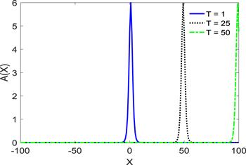
From figure 1, we can see that solitary waves have the classical bell shape, and the shape does not change with time. This shows that equations (41) and (42) are the single solitary wave solutions of equation (37).
Figure 1. Equation (41) is presented as a single solitary wave with $a=k=l=Y=1,b=-1,{\alpha }_{1}=1,{\alpha }_{2}=\tfrac{1}{2}$ and ${\alpha }_{3}=\tfrac{3}{2}$.

3.2. Asymptotic solitary wave solution of the forced ZK–Burgers equation

First, equation (28) is considered with dissipation but without topography, as follows:
$\begin{eqnarray}\displaystyle \frac{\partial A}{\partial T}+{\alpha }_{1}A\displaystyle \frac{\partial A}{\partial X}+{\alpha }_{2}\displaystyle \frac{{\partial }^{3}A}{\partial {X}^{3}}+{\alpha }_{3}\displaystyle \frac{{\partial }^{3}A}{\partial X\partial {Y}^{2}}+\eta A=0.\end{eqnarray}$
When $\eta \ll 1$, the asymptotic solitary wave solution of equation (43) is obtained using a new modified ansatz method. Assuming that the solution of equation (44) is as follows:
$\begin{eqnarray}A(X,Y,T)={A}_{0}{{\rm{{\rm{sech}} }}}^{p}\theta ,\end{eqnarray}$
where ${A}_{0}={A}_{0}(T),\theta =k(T)[(X+Y)-\nu (T)]$, and p is a non-negative integer to be determined. Substituting equation (44) into equation (45), we obtain
$\begin{eqnarray}\begin{array}{l}\displaystyle \frac{{\rm{d}}{A}_{0}}{{\rm{d}}T}{{\rm{{\rm{sech}} }}}^{p}\theta -{{pA}}_{0}{{\rm{{\rm{sech}} }}}^{p}\theta \tanh \theta \left[\displaystyle \frac{{\rm{d}}k}{{\rm{d}}T}(X+Y-\nu )-k\displaystyle \frac{{\rm{d}}\nu }{{\rm{d}}T}\right]\\ -\,{\alpha }_{1}{{pA}}_{0}^{2}k{{\rm{{\rm{sech}} }}}^{2p}\theta \tanh \theta -{\alpha }_{2}{p}^{3}{A}_{0}{k}^{3}{{\rm{{\rm{sech}} }}}^{p}\theta \tanh \theta \\ -\,{\alpha }_{2}p(p+1)(p+2){A}_{0}{k}^{3}{{\rm{{\rm{sech}} }}}^{p+2}\theta \tanh \theta \\ -\,{\alpha }_{3}{p}^{3}{A}_{0}{k}^{3}{{\rm{{\rm{sech}} }}}^{p}\theta \tanh \theta \\ -\,{\alpha }_{3}p(p+1)(p+2){A}_{0}{k}^{3}{{\rm{{\rm{sech}} }}}^{p+2}\theta \tanh \theta \\ +\,\eta {A}_{0}{{\rm{{\rm{sech}} }}}^{p}\theta =0.\end{array}\end{eqnarray}$
Matching the exponents of ${{\rm{{\rm{sech}} }}}^{2p}\theta $ and ${{\rm{{\rm{sech}} }}}^{p+2}\theta $ in equation (45), we obtain
$\begin{eqnarray}p=2.\end{eqnarray}$
We set the coefficients of the ${{\rm{{\rm{sech}} }}}^{p}\theta ,{{\rm{{\rm{sech}} }}}^{p}\theta \tanh \theta $ and ${{\rm{{\rm{sech}} }}}^{2p}\theta \tanh \theta $ terms to zero. This leads to
$\begin{eqnarray}\displaystyle \frac{{\rm{d}}{A}_{0}}{{\rm{d}}T}+\eta {A}_{0}=0,\end{eqnarray}$
$\begin{eqnarray}\begin{array}{l}-{{pA}}_{0}\left[\displaystyle \frac{{\rm{d}}k}{{\rm{d}}T}(X+Y-\nu )-k\displaystyle \frac{{\rm{d}}\nu }{{\rm{d}}T}\right]\\ \quad -\,{\alpha }_{2}{p}^{3}{A}_{0}{k}^{3}-{\alpha }_{3}{p}^{3}{A}_{0}{k}^{3}=0,\end{array}\end{eqnarray}$
$\begin{eqnarray}\begin{array}{l}-{\alpha }_{1}{{pA}}_{0}^{2}k+{\alpha }_{2}p(p+1)(p+2){A}_{0}{k}^{3}\\ \quad +\,{\alpha }_{3}p(p+1)(p+2){A}_{0}{k}^{3}=0.\end{array}\end{eqnarray}$
From equations (47) and (49) we obtain
$\begin{eqnarray}{A}_{0}(T)=\overline{{A}_{0}}{{\rm{e}}}^{-\eta T},k(T)={\left[\displaystyle \frac{{\alpha }_{1}\overline{{A}_{0}}}{12({\alpha }_{2}+{\alpha }_{3})}\right]}^{\tfrac{1}{2}}{{\rm{e}}}^{-\tfrac{\eta }{2}T},\end{eqnarray}$
where $\overline{{A}_{0}}={A}_{0}(T=0)=\tfrac{3c}{{\alpha }_{1}}$. Substituting equation (50) into equation (48) yields
$\begin{eqnarray}-\displaystyle \frac{\eta }{2}(X+Y-\nu )-\displaystyle \frac{{\rm{d}}\nu }{{\rm{d}}T}+\displaystyle \frac{{\alpha }_{1}\overline{{A}_{0}}}{3}{{\rm{e}}}^{-\eta T}=0.\end{eqnarray}$
As $\eta \ll 1$, the term $-\tfrac{\eta }{2}(X+Y-\nu )$ can be omitted in equation (51). Accordingly
$\begin{eqnarray}\nu ={\int }_{0}^{T}\displaystyle \frac{{\alpha }_{1}\overline{{A}_{0}}}{3}{{\rm{e}}}^{-\eta T}{\rm{d}}T=0.\end{eqnarray}$
So, we get the asymptotic solitary wave solution of equation (43) as follows:
$\begin{eqnarray}\begin{array}{l}A(X,Y,T)\approx \overline{{A}_{0}}{{\rm{e}}}^{-\eta T}{{\rm{{\rm{sech}} }}}^{2}\\ \times \,\left\{{\left[\displaystyle \frac{{\alpha }_{1}\overline{{A}_{0}}}{12({\alpha }_{2}+{\alpha }_{3})}\right]}^{\tfrac{1}{2}}{{\rm{e}}}^{-\tfrac{\eta }{2}T}(X+Y-{\displaystyle \int }_{0}^{T}\displaystyle \frac{{\alpha }_{1}\overline{{A}_{0}}}{3}{{\rm{e}}}^{-\eta T}{\rm{d}}T)\right\}.\end{array}\end{eqnarray}$
The velocity and width of a solitary wave are obtained, respectively,
$\begin{eqnarray}{C}_{s}=\displaystyle \frac{{\alpha }_{1}\overline{{A}_{0}}}{3}{{\rm{e}}}^{-\eta T},{W}_{s}={\left[\displaystyle \frac{12({\alpha }_{2}+{\alpha }_{3})}{{\alpha }_{1}}\right]}^{\tfrac{1}{2}}{\overline{{A}_{0}}}^{-\tfrac{1}{2}}{{\rm{e}}}^{\tfrac{\eta }{2}T}.\end{eqnarray}$
Second, we seek the asymptotic solitary wave solution of equation (28) with dissipation and topographic forcing. To simplify the calculation, and to consider that the variation of topography with time is much smaller than that with the meridional direction in large-scale atmospheric and oceanic motion, we assume slowly varying topography as:
$\begin{eqnarray}\displaystyle \frac{\partial H(X,T)}{\partial X}={\delta }_{0},\end{eqnarray}$
where ${\delta }_{0}\ll 1$ are small parameters that describe the variation in the degree of topography with meridional direction. Equation (55) is called the slowly varying linear topography. We perform the following transformation:
$\begin{eqnarray}A(X,Y,T)=B(X,Y,T)+\displaystyle \frac{\gamma {\delta }_{0}}{\eta }.\end{eqnarray}$
Substituting equations (55) and (56) into equation (28) yields
$\begin{eqnarray}\begin{array}{l}\displaystyle \frac{\partial B}{\partial T}+{\alpha }_{1}B\displaystyle \frac{\partial B}{\partial X}+{\alpha }_{1}\displaystyle \frac{\gamma {\delta }_{0}}{\eta }\displaystyle \frac{\partial B}{\partial X}\\ \quad +\,{\alpha }_{2}\displaystyle \frac{{\partial }^{3}B}{\partial {X}^{3}}+{\alpha }_{3}\displaystyle \frac{{\partial }^{3}B}{\partial X\partial {Y}^{2}}+\eta B=0.\end{array}\end{eqnarray}$
Further, introducing the transformation $T^{\prime} =T,X^{\prime} \,=X-{\alpha }_{1}\tfrac{\gamma {\delta }_{0}}{\eta }T,Y^{\prime} =Y$, substituting the transformation into equation (57) and omitting the apostrophe, we rewrite equation (57) in the following form:
$\begin{eqnarray}\displaystyle \frac{\partial B}{\partial T}+{\alpha }_{1}B\displaystyle \frac{\partial B}{\partial X}+{\alpha }_{2}\displaystyle \frac{{\partial }^{3}B}{\partial {X}^{3}}+{\alpha }_{3}\displaystyle \frac{{\partial }^{3}B}{\partial X\partial {Y}^{2}}+\eta B=0.\end{eqnarray}$
Noting that equation (58) is in the same form as equation (43), we can obtain the asymptotic solitary wave solution of equation (28) with slowly varying topography (55).
$\begin{eqnarray}\begin{array}{l}A(X,Y,T)\approx \displaystyle \frac{\gamma {\delta }_{0}}{\eta }+\overline{{A}_{0}}{{\rm{e}}}^{-\eta T}{{\rm{{\rm{sech}} }}}^{2}\left\{{\left[\displaystyle \frac{{\alpha }_{1}\overline{{A}_{0}}}{12({\alpha }_{2}+{\alpha }_{3})}\right]}^{\tfrac{1}{2}}{{\rm{e}}}^{-\eta /2T}\right.\\ \qquad \left.\times \left(X+Y-\displaystyle \frac{{\alpha }_{1}\gamma {\delta }_{0}}{\eta }T-{\displaystyle \int }_{0}^{T}\displaystyle \frac{{\alpha }_{1}\overline{{A}_{0}}}{3}{{\rm{e}}}^{-\eta T}{\rm{d}}T\right)\right\}.\end{array}\end{eqnarray}$
The velocity of the solitary wave is
$\begin{eqnarray}{C}_{s}=\displaystyle \frac{{\alpha }_{1}\overline{{A}_{0}}}{3}{{\rm{e}}}^{-\eta T}+\displaystyle \frac{{\alpha }_{1}\gamma {\delta }_{0}}{\eta }.\end{eqnarray}$
From equations (53), (54), (59) and (60), it is evident that dissipation and slowly varying topography affect the amplitude and velocity and width of solitary waves.
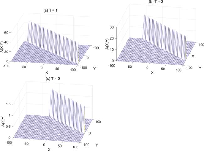
From figure 2, It can be found that the topography weakly affects the amplitude of solitary waves when T = 1 and T = 3. However, when T = 5, the amplitude of solitary waves increases slightly because of slowly varying topography. This shows that dissipation and slowly varying topography affect the formation of solitary waves. This is consistent with asymptotic solutions (59).
Figure 2. The asymptotic solitary wave solution of equation (28) with parameters $\eta =0.01,{\delta }_{0}=0.01,\gamma =1,{\alpha }_{1}=1,{\alpha }_{2}=\tfrac{1}{2}$ and ${\alpha }_{3}=\tfrac{3}{2}$.

4. Conclusion

We derive the (2+1)-dimensional ZK–Burgers equation based on the dimensionless quasi-geostrophic potential vorticity equation by using multiple scales and the perturbation expansion method; this is a high-dimensional mathematical model for describing nonlinear Rossby waves in stratified fluid for the first time. Also, we analyze the effects of the generalized beta, dissipation and topography on the solitary waves. We conclude that basic topography is an essential factor; basic topography and the generalized beta can induce nonlinear waves. The mass and energy of solitary waves are conserved when without dissipation and slowly varying topography. Moreover, we obtain the single solitary wave solution for the ZK–Burgers equation in the absence of dissipation and topography, which is a classical bell solitary wave solution. We obtain asymptotic solitary wave solution of the forced ZK-Bergurs equation with small dissipation and slowly varying linear topography by a new modified ansatz method. The results of the solitary wave solutions show that the dissipation can cause the velocity and amplitude of solitary waves to decrease exponentially with time, but opposite to the width of solitary waves. Furthermore, slowly varying linear topography can affect the velocity of solitary waves, while it does not significantly influence the amplitude of solitary waves when time is short. As time increases, slowly varying linear topography affects the formation of solitary waves. In the previous study, we have only considered the slowly varying linear topography. For the general varying topography, we will conduct further study in future work. In addition, the numerical calculation of the model is our next research work.
1
Russell J S 1837 Tech. Rep. Brit. Assoc. Adv. Sci. 41 331

2
Wang D S Shi Y R Feng W X Wen L 2017 Phys. D 351–352 30

DOI

3
Wang D S Song S W Xiong B Liu W M 2011 Phys. Rev. A 84 053607

DOI

4
Wang D S Zhang D J Yang J 2010 J. Math. Phys. 51 023510

DOI

5
Korteweg D J de Vries G 1895 Phil. Mag. 39 442

DOI

6
Zedan H A Aladrous E Shapll S 2013 Nonlinear Dyn. 74 1145

DOI

7
Wang M I Zhou Y Li Z 1996 Phys. Lett. A 216 67

DOI

8
Fu Z T Li S K Liu S D Zhao Q 2001 Phys. Lett. A 290 72

DOI

9
Hereman W Nuseir A 1997 Math. Comput. Simul. 43 13

DOI

10
Liu S K Fu Z T Liu S D Zhao Q 2001 Phys. Lett. A 289 69

DOI

11
Maxworthy T Redekopp L G 1976 Nature 260 509

DOI

12
Luo D H Ji L R 1989 Sci. China. 33 323 (in Chinese)

13
Horel J D Wallace J M 1981 Mon. Weather. Rev. 109 813

DOI

14
Ambrizzi T Hoskins B J Hsu H H 1995 J. Atmos. Sci. 52 3661

DOI

15
Long R R 1964 J. Atmos. Sci. 21 197

DOI

16
Wadati M 1973 J. Phys. Soc. Jpn. 34 1289

DOI

17
Redekopp L G 1977 J. Fluid. Mech. 82 725

DOI

18
Grimshaw R 1977 Geophys. Astro. Fluid. Dyn. 8 3

DOI

19
Benney D J 1966 J. Math. Phys. 45 52

DOI

20
Redekopp L G Weidman P D 1978 J. Atmos. Sci. 35 790

DOI

21
Meng L Lv K L 2002 Chin J. Comput. Phys. 19 89

22
Boyd J P 1980 J. Phys. Ocean. 10 1699

DOI

23
Boyd J P 1983 J. Phys. Ocean. 13 428

DOI

24
Le K C Nguyen L T K 2014 Int. J. Eng. Sci. 83 117

DOI

25
Ono H 1981 J. Phys. Soc. Jpn. 50 2757

DOI

26
Luo D H 1989 Sci. China Ser. B 32 1233

27
Jiang H S Lv K L 1989 Plateau. Meteorology 17 231 (in Chinese)

28
Meng L Lv K L 2002 Chin. J. Comput. Phys. 19 259

29
Yang H W Zhao Q Yin B S Dong H H 2013 Abstr. Appl. Anal. 2013 597807

30
Yang H W Yin B S Shi Y L Wang Q B 2012 J. Appl. Math. 2012 491343

31
Yang H W Yang D Z Shi Y L Yin B S 2015 Dyn. Atmos. Oceans. 17 21

DOI

32
Guo M Zhang Y Wang M Chen Y D Yang H W 1980 Comput. Math. App. 10 1699

33
Yang H W Wang X R Yin B S 2014 Nonlinear. Dyn. 76 1725

DOI

34
Yin X J Yang L G Liu Q S Su J M Wu G R 2018 Chaos. Solitons. Fractals. 111 68

DOI

35
Liu S K Tan B K 1992 Appl. Math. Mech. 13 35

36
Song J Yang L G 2009 Chin. Phys. B 18 2873

DOI

37
Song J Liu Q S Yang L G 2012 Acta. Phys. Sin. 61 210510 (in Chinese)

38
Li S F Yang L G Song J 2015 Acta. Phys. Sin. 64 199 (in Chinese)

39
Gottwalld G A 2009 2013 (arXiv:org/abs/nlin/031)

40
Yang H W Xu Z H Yang D Z Feng X R Yin B S Dong H H 2016 Adv. Differ. Equ. 2016 167

DOI

41
Zhao B J Wang R Y Sun J W Yang H W 2018 Adv. Differ. Equ. 2018 42

DOI

42
Zhang R G Yang L G Song J Liu Q S 2017 Nonlinear. Dyn. 90 815

DOI

43
Zhang R G Yang L G Song J Yang H L 2017 Comput. Math. App. 73 1996

44
Liu Q S Zhang Z Y Zhang R G Huang C X 2019 Commun. Theor. Phys. 71 1054

DOI

45
Chen L G Yang L G Zhang R G Cui J F 2019 Results. Phys. 13 102280

DOI

46
Lu C N Fu C Yang H W 2018 Appl. Math. Comput. 327 104

DOI

47
Meng L Lv K L 2002 Chin J. Comput. Phys. 19 349

DOI

48
Zhao B J Wang R Y Fang Q Sun W J Zhan T M 2017 Nonlinear Dyn. 90 889

DOI

49
Luo D H 1990 Adv. Atmos. Sci. 7 433

DOI

50
Da C J Chou J F 2008 Acta. Phys. Sin. 57 2595 (in Chinese).

51
Song J Yang L G Liu Q S 2014 Acta Phys. Sin. 63 060401 (in Chinese)

52
Ren Y W Tao M S Dong H H Yang H W 2019 Adv. Differ. Equ. 2019 13

DOI

53
Yang H W Guo M He H 2018 Int. J. Nonlin. Sci. Num. 20 0026

54
Fu C Lu C N Yang H W 2018 Adv. Differ. Equ. 2018 56

DOI

55
Fu L Chen Y D Yang H W 2019 Mathematics 7 41

DOI

56
Yang H W Sun J C Fu C 2019 Commun. Non. Sci. Numer. Simu. 71 187

DOI

57
Lu C N Xie L Y Yang H W 2019 Comput. Math. App. 77 3154

58
Song F X Yu Z Y Yang H W 2019 Math. Model. Nat. Pheno. 14 301

DOI

59
Tian R H Fu L Ren Y W Yang H W 2019 Math. Meth. Appl. Sci. 2019 1

60
Guo M Dong H Y Liu J X Yang H W 2019 Nonlinear Anal.: Model. Contr. 24 1

DOI

61
Pedlosky J 1979 Geophysical Fluid Dynamics New York Springer

62
Yin Y H Ma W X Liu J G X 2018 Comput. Math. App. 76 1275

DOI

63
Kuo C K 2018 Comput. Math. App. 75 2851

DOI

64
Wazwaz A M 2015 Commun. Nonlinear. Sci. Numer. Simul. 10 597

DOI

65
Taghizadeh N Mirzazadeh M 2011 Internat. J. Appl. Math. Comput. 3 151

66
Gao L N Zi Y Y Yin Y H Ma W X X 2017 Nonlinear. Dyn. 89 2233

DOI

Outlines

/