


1. Introduction
Entropic measures and information theory in general provides a clear understanding of quantum mechanical systems. In recent years, the study of bound state and scattering state solutions for both relativistic and non-relativistic wave equations has a gained wider interest because of their potential applications, particularly in the areas of information entropies and quantum technologies. Information entropy is a significant tool in studying the electronic structure of atoms and molecules. The Fisher information measurement is used as a tool for characterising complex signals of quantum mechanical systems with applications to biology, atomic physics and other related science disciplines [1–13]. Shannon, Fisher and other quantum information entropies usually measure the spread of probability distribution for allowed quantum mechanical states in a D-dimensional space [14–18]. Quantum information theory has a direct relationship with the Heisenberg uncertainty principle, which plays a very significant role in the simultaneous measurement of position and momentum of quantum mechanical particles. In 1948, a new uncertainty relation, based on Shannon entropy, was established as a basic tool for investigating the fundamental limit of signal processing [19, 20]. In this work, we developed a novel potential called a Noncentral Inversely Quadratic plus exponential Mie-type potential to study Fisher and and Shannon entropies, their expectation values, and their squeeze state, using suitable real constant parameters. This potential has applications in signal processing. The wave function and probability density plots obtained in this work reveal some significant properties and characteristics of quantum systems. We have discovered that all odd values of the wave function give the property of a wave function, while even values of the wave function plots give probability density. Larger values of the Shannon entropy are indicative of a more delocalised density while smaller values are associated with localised distribution. This means that Shannon entropy increases with an increase in uncertainty and vice versa [21]. There are other information entropies as investigated by various researchers. Recently Jen-Hao and Yew Ho carried out fantastic work on the benchmark calculations of Renyi, Tsallis and Onicescu information entropies for ground state helium using a correlated Hylleraas wave function [22]. The new Shannon entropy was first introduced by Beckner, Bialynicki-Birula and Mycieslki in 1975 as ${S}_{x}+{S}_{p}\geqslant D(1+{log}\pi )$ [23–25] where D represents the spatial dimension. However, the position Sx and momentum Sp is defined as [26–29].1 ) and (2 ) give the measure of the spread of a single particle density of position and momentum space respectively. Equation (1 ) and (2 ) can also be expressed as3 ) can further be expressed as1 gives a brief introduction of the article. In section 2 , we provide an overview of the generalised parametric Nikiforov–Uvarov method. In section 3 we solve analytically the radial solution of a Schrödinger wave equation to obtain a normalised wave function and the energy-eigen equation. In section 4 we apply the normalised wave function obtained in section 3 to analytically obtained position and momentum space Shannon entropy. In section 5 , we obtain analytical solutions to Fisher position and momentum space entropies. We present the numerical solutions , their expectation values and the squeeze state in section 6 . Results and discussion are presented in section 7 while section 8 gives the conclusion of the article. The adopted parameter values for both the wave function and probability density plots were all real constants. We discover that the proposed potential is most suitable for ground state energy. This is a further reason why our plots for wave functions and probability densities are all plotted for n, l = 0 using a well designed rigorous mathematica algorithm. We also discover that at higher state, that is for n, l > 0, The plots were not suitable in providing solutions to the information measures of Shannon and Fisher entropies for this particular potential. Therefore, this work is limited to ground state energy and wave function. The normalisation constant, the wave function plots, the probability density plots, and all numerical computations were carried out using Mathematica. The graph for the noncentral potential is given in figure 1, while that of the Greene Aldrich approximation and special Greene Aldrich approximation are presented in figures 1(a) and (b) respectively. The combination of the noncentral and exponential Mie-type potential is significant in the study of vibrational and rotational energies of diatomic molecules and their degeneracies for a particular quantum state [32]. In most cases, the topological properties of atoms of diatomic molecules, including their chemical functional groups, are evaluated using Density Functional theory(DFT) and pseudopotential formalism [33]. Inversely quadratic potential is a long range potential and in combination with other exponential type potentials may be used in finding the shape of organic molecules such as cyclic polyenes and benzene [22].
$\begin{eqnarray}{S}_{x}=-{\int }_{-\infty }^{+\infty }{\left|{\rm{\Psi }}(x)\right|}^{2}\mathrm{log}{\left|{\rm{\Psi }}(x)\right|}^{2}{\rm{d}}{x}\end{eqnarray}$
$\begin{eqnarray}{S}_{p}=-{\int }_{-\infty }^{+\infty }{\left|\phi (p)\right|}^{2}\mathrm{log}{\left|\phi (p)\right|}^{2}{\rm{d}}{p}\end{eqnarray}$
where &PSgr;(x) is a normalised eigen function in a spatial coordinate and φ(x) is the normalised Fourier transform. In general, the momentum space entropy is obtained by taking the Fourier transform of position space in a spatial coordinate [30, 31]. Equations ( $\begin{eqnarray}{S}_{x}=-{\int }_{-\infty }^{+\infty }\rho (x)\mathrm{ln}\rho (x){\rm{d}}{x}\end{eqnarray}$
$\begin{eqnarray}{S}_{p}=-{\int }_{-\infty }^{+\infty }\rho (p)\mathrm{ln}\rho (p){\rm{d}}{p},\end{eqnarray}$
where $\rho (x)={\left|{\rm{\Psi }}(x)\right|}^{2}$ and $\rho (p)={\left|{\rm{\Psi }}(p)\right|}^{2}$ respectively. Equation ( $\begin{eqnarray}\begin{array}{rcl}{S}_{x} & = & -{\displaystyle \int }_{-\infty }^{+\infty }\left(\displaystyle \frac{1}{{d}^{2}}{\left|{P}_{n}(x)\right|}^{2}w(x\right)\\ & & \times \mathrm{log}\left(\displaystyle \frac{1}{{d}^{2}}{\left|{P}_{n}(x)\right|}^{2}w(x\right){\rm{d}}{x},\end{array}\end{eqnarray}$
where $\begin{eqnarray}{S}_{x}=\mathrm{log}({{\rm{d}}}_{n}^{2})+\displaystyle \frac{1}{{{\rm{d}}}^{2}}\left({E}_{n}+{I}_{n}\right).\end{eqnarray}$
Here, the term En and In can then be expressed as $\begin{eqnarray}{E}_{n}=-{\int }_{-\infty }^{+\infty }\left({\left|{P}_{n}(x)\right|}^{2}w(x\right)\mathrm{log}\left({\left|{P}_{n}(x)\right|}^{2}\right){\rm{d}}{x},\end{eqnarray}$
$\begin{eqnarray}{I}_{n}=-{\int }_{-\infty }^{+\infty }\left({\left|{P}_{n}(x)\right|}^{2}w(x\right)\mathrm{log}\left(w(x\right){\rm{d}}{x}.\end{eqnarray}$
This work is divided into seven sections. Section 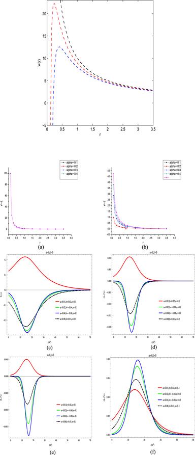
Figure 1. The graph of the Noncentral potential. (a) The centrifugal term $\tfrac{1}{{r}^{2}}$ for standard Greene Aldrich approximation with varying α = 0.1 to 0.5. (b) The centrifugal term $\tfrac{1}{{r}^{2}}$ for special Greene Aldrich approximation with varying α = 0.1 to 0.5. (c) The normalised wave function plot 1. (d) The normalised wave function plot 2. (e) The normalised wave function plot 3. (f) The probability density function plot 1. (g) The probability density function plot 2. (h) The probability density function plot 3. (i) The normalised wave function plot 1(a). (j) The normalised wave function plot 2(a). (k) The normalised wave function plot 3(a). (l) The probability density function plot 1(b). (m) The probability density function plot 2(b). (n) The probability density function plot 3(b). |
2. The generalised parametric Nikiforov–Uvarov method
The NU method was presented by Nikiforov and Uvarov [31] and has been employed to solve second order differential equations such as Schrödinger wave equations (SWE), Klein–Gordon equations (KGE), Dirac equations (DE), etc. The Schrödinger wave equation is given as9 ) reduces to10 ) can be solved by transforming it into an hypergeometric type equation using the transformation s = s(x) and its resulting equation is expressed as:12 .12 ) has been applied to provide bound state solutions to both relativistic and non-relativistic wave equations with considerable potential such as Hulthen, Eckart, Coulomb, Pseudoharmonic and many others [34–41]. Equation (12 ) is solved by comparing with equation (11 ) and the following polynomials are obtained.
$\begin{eqnarray}\displaystyle \frac{{{\rm{d}}}^{2}{\rm{\Psi }}(r)}{{{\rm{d}}{r}}^{2}}+\displaystyle \frac{2\mu }{{{\hslash }}^{2}}\left[{E}_{{nl}}-V(r)-\displaystyle \frac{{{\hslash }}^{2}l(l+1)}{2\mu {r}^{2}}\right]{\rm{\Psi }}(r)=0,\end{eqnarray}$
correspondingly, for the purpose of this work, we shall be considering the exact solution of a Schrödinger equation where the orbital angular quantum number l = 0, hence equation ( $\begin{eqnarray}\displaystyle \frac{{{\rm{d}}}^{2}{\rm{\Psi }}(r)}{{{\rm{d}}{r}}^{2}}+\displaystyle \frac{2\mu }{{{\hslash }}^{2}}\left[{E}_{{nl}}-V(r)\right]{\rm{\Psi }}(r)=0.\end{eqnarray}$
Equation ( $\begin{eqnarray}\psi ^{\prime\prime} (s)+\displaystyle \frac{\tilde{\tau }(s)}{\sigma (s)}\psi ^{\prime} (s)+\displaystyle \frac{\tilde{\sigma }(s)}{{\sigma }^{2}(s)}\psi (s)=0,\end{eqnarray}$
where σ (s) and $\tilde{\sigma }(s)$ must be polynomials of at most second degree, $\tilde{\tau }(s)$ is the first degree polynomial, and ψ (s) is a function of the hypergeometric type. The parametric generalisation of the NU method is given by the generalised hypergeometric type equation $\begin{eqnarray}\begin{array}{l}\psi ^{\prime\prime} (s)+\displaystyle \frac{({c}_{1}-{c}_{2}s)}{s(1-{c}_{3}s)}\psi ^{\prime} (s)\\ \quad +\,\displaystyle \frac{1}{{s}^{2}{\left(1-{c}_{3}s\right)}^{2}}\left[-{\xi }_{1}{s}^{2}+{\xi }_{2}s-{\xi }_{3}\right]\psi (s)=0.\end{array}\end{eqnarray}$
Equation ( $\begin{eqnarray}\begin{array}{rcl}\tilde{\tau }(s) & = & \left({c}_{1}-{c}_{2}s\right),\sigma (s)=s\left(1-{c}_{3}s\right),\\ \tilde{\sigma }(s) & = & -{\epsilon }_{1}{s}^{2}+{\epsilon }_{2}s-{\epsilon }_{3}.\end{array}\end{eqnarray}$
According to the NU method, the energy eigenvalue equation and eigen wave function, respectively, satisfy the following set of equations: $\begin{eqnarray}\begin{array}{l}{c}_{2}^{}n-\left(2n+1\right){c}_{5}\left(2n+1\right)\left(\sqrt{{c}_{9}}+{c}_{3}\sqrt{{c}_{8}}\right)\\ \quad +\,n\left(n-1\right){c}_{3}+{c}_{7}2{c}_{3}{c}_{8}+2\sqrt{{c}_{8}{c}_{9}}=0,\end{array}\end{eqnarray}$
$\begin{eqnarray}\psi (s)={N}_{{nl}}{s}^{{c}_{12}}{\left(1-{c}_{3}s\right)}^{-{c}_{12}-\tfrac{{c}_{11}}{{c}_{3}}}{P}_{n}^{\left({c}_{10}-1,\,\tfrac{{c}_{11}}{{c}_{3}}-{c}_{10}-1\right)}\left(1-2{c}_{3}s,,\right)\end{eqnarray}$
where $\begin{eqnarray}\left.\begin{array}{l}\,{c}_{4}=\displaystyle \frac{1}{2}\left(1-{c}_{1}\right);\,{c}_{5}=\displaystyle \frac{1}{2}\left({c}_{2}-{c}_{3}\right);\,{c}_{6}={c}_{5}^{2}+{\epsilon }_{1}\\ \,{c}_{7}=2{c}_{4}{c}_{5}-{\epsilon }_{2};\,{c}_{8}={c}_{4}^{2}+{\epsilon }_{3};\\ \,{c}_{9}={c}_{3}{c}_{7}+{c}_{3}^{2}{c}_{8}+{c}_{6}\\ {c}_{10}={c}_{1}+2{c}_{4}+2\sqrt{{c}_{8}};\\ {c}_{11}={c}_{2}-2{c}_{5}+2\left(\sqrt{{c}_{9}}+{c}_{3}\sqrt{{c}_{8}}\right)\\ {c}_{12}={c}_{4}+\sqrt{{c}_{8}};\,{c}_{13}={c}_{5}-\left(\sqrt{{c}_{9}}+{c}_{3}\sqrt{{c}_{8}}\right)\end{array}\right\}.\end{eqnarray}$
3. The radial solution of the proposed potential in a Schrödinger equation using the Nikiforov–Uvarov method
The noncentral Inversely quadratic plus exponential Mie-type potential is given as
$\begin{eqnarray}V(r)=\displaystyle \frac{A\sin \alpha }{{r}^{2}}+\displaystyle \frac{\left(B-\eta \right){{\rm{e}}}^{-\alpha r}\sin \alpha }{r}+C,\end{eqnarray}$
where A is the potential depth in electron volts, B, η and C are real constant parameters. α is the screening parameter. The graph of this potential is shown in figure 1.Substituting equation (17 ) into (10 ) gives18 ) analytically, we treat sin $\alpha $ as a constant trignometric function that tends to 1 and define special Greene Aldrich approximation to the centrifugal term as
$\begin{eqnarray}\begin{array}{l}\displaystyle \frac{{{\rm{d}}}^{2}{\rm{\Psi }}(r)}{{{\rm{d}}{r}}^{2}}+\displaystyle \frac{2\mu }{{{\hslash }}^{2}}\left[{E}_{{nl}}-\displaystyle \frac{A\sin \alpha }{{r}^{2}}\right.\\ \quad \left.-\,\displaystyle \frac{\left(B-\eta \right){{\rm{e}}}^{-\alpha r}\sin \alpha }{r}-C\right]{\rm{\Psi }}(r)=0.\end{array}\end{eqnarray}$
To solve equation ( $\begin{eqnarray}\displaystyle \frac{1}{{r}^{2}}=\displaystyle \frac{4{\alpha }^{2}{{\rm{e}}}^{-2\alpha r}\sin \alpha }{{\left(1-{{\rm{e}}}^{-2\alpha r}\sin \alpha \right)}^{2}}\Rightarrow \displaystyle \frac{1}{r}=\displaystyle \frac{2\alpha {{\rm{e}}}^{-\alpha r}\sin \alpha }{\left(1-{{\rm{e}}}^{-2\alpha r}\sin \alpha \right)}.\end{eqnarray}$
Let us define a special transformation to S-coordinate as19 ) into 18 , and making use of equation (20 ), equation (18 ) is reduced to a hypergeometric type equation:12 ) to equation (21 ), and using equation (16 ), the following parametric constants are obtained:14 ), the energy-eigen equation for the proposed potential is given as15 ), the total wave function is given as
$\begin{eqnarray}s={{\rm{e}}}^{-2\alpha r}\sin \alpha .\end{eqnarray}$
By comparing the graph of a standard Greene Aldrich approximation in figure 1(a) to a special Greene Aldrich approximation in figure 1(b), it can be observed that figure 1(a) converges asymptotically for different values of the screening parameter α = 0.1 to 0.5. The same thing is also applicable to figure 1(b). This signifies that the special Greene Aldrich approximation could be approximated to the standard Greene Aldrich approximation; this serves as a good approximation to the proposed potential. Substituting equation ( $\begin{eqnarray}\begin{array}{l}\displaystyle \frac{{{\rm{d}}}^{2}{\rm{\Psi }}(s)}{{{\rm{d}}{s}}^{2}}+\displaystyle \frac{(1-s)}{s(1-s)}\displaystyle \frac{{\rm{d}}{\rm{\Psi }}(s)}{{\rm{d}}{s}}+\displaystyle \frac{1}{s(1-s)}\\ \times \,\left[\begin{array}{l}-\left({\varepsilon }^{2}+{\chi }_{2}+{\chi }_{3}\right){s}^{2}+\left(2{\varepsilon }^{2}-{\chi }_{1}-{\chi }_{2}+2{\chi }_{3}\right)s\\ -\left({\varepsilon }^{2}+{\chi }_{3}\right)\end{array}\right]\\ \times \,{\rm{\Psi }}(s)=0,\end{array}\end{eqnarray}$
where $\begin{eqnarray}\begin{array}{rcl}{\chi }_{1} & = & \displaystyle \frac{\mu A}{{{\hslash }}^{2}}\ ;\ {\chi }_{2}=\displaystyle \frac{\mu \left(B-\eta \right)}{\alpha {{\hslash }}^{2}}\ ;\ {\chi }_{3}=\displaystyle \frac{2\mu C}{4{\alpha }^{2}{{\hslash }}^{2}};\\ {\varepsilon }^{2} & = & -\displaystyle \frac{2\mu {E}_{{nl}}}{4{\alpha }^{2}{{\hslash }}^{2}}.\end{array}\end{eqnarray}$
Comparing equation ( $\begin{eqnarray}\begin{array}{l}{c}_{1}={c}_{2}={c}_{3}=1;\ \ {c}_{4}=0;\\ {c}_{5}=-\displaystyle \frac{1}{2};\ \ {c}_{6}=\displaystyle \frac{1}{4}+{\varepsilon }^{2};\\ {c}_{7}=\left(-2{\varepsilon }^{2}+{\chi }_{1}+{\chi }_{2}-2{\chi }_{3}\right);\\ {c}_{8}=\left({\varepsilon }^{2}+{\chi }_{3}\right);\ \ {c}_{9}=\left(\displaystyle \frac{1}{4}+{\chi }_{1}+2{\chi }_{2}\right);\\ {c}_{10}=\left(1+2\sqrt{{\varepsilon }^{2}+{\chi }_{3}}\right);\\ {c}_{11}=2+2\left(\sqrt{\displaystyle \frac{1}{4}+{\chi }_{1}+2{\chi }_{2}}+\sqrt{{\varepsilon }^{2}+{\chi }_{3}}\right);\\ {c}_{12}=\sqrt{{\varepsilon }^{2}+{\chi }_{3}};\\ {c}_{13}=-\displaystyle \frac{1}{2}-\left(\sqrt{\displaystyle \frac{1}{4}+{\chi }_{1}+2{\chi }_{2}}+\sqrt{{\varepsilon }^{2}+{\chi }_{3}}\right);\\ {\xi }_{1}=\left({\varepsilon }^{2}+{\chi }_{2}+{\chi }_{3}\right);\\ {\xi }_{2}=\left(2{\varepsilon }^{2}-{\chi }_{1}-{\chi }_{2}+2{\chi }_{3}\right);\ \ {\xi }_{3}=\left({\varepsilon }^{2}+{\chi }_{3}\right).\end{array}\end{eqnarray}$
By making use of equation ( $\begin{eqnarray}\begin{array}{c}\begin{array}{l}{E}_{{nl}}=\displaystyle \frac{-2{\alpha }^{2}{\hslash }^{2}}{\mu }\times \,{\left\{\displaystyle \frac{\left({n}^{2}+n+\tfrac{1}{2}\right)+\left(n+\tfrac{1}{2}\right)\sqrt{1+\tfrac{4\mu A}{{\hslash }^{2}}+\tfrac{8\mu \left(B-\eta \right)}{\alpha {\hslash }^{2}}}+\tfrac{\mu A}{{\hslash }^{2}}+\tfrac{\mu \left(B-\eta \right)}{\alpha {\hslash }^{2}}}{\left(2n+1\right)+\sqrt{1+\tfrac{4\mu A}{{\hslash }^{2}}+\tfrac{8\mu \left(B-\eta \right)}{\alpha {\hslash }^{2}}}}\right\}}^{2}+\,C.\end{array}\end{array}\end{eqnarray}$
Also, by making use of equation ( $\begin{eqnarray}\begin{array}{l}{{\rm{\Psi }}}_{n}(s)={N}_{n}{S}^{\sqrt{{\varepsilon }^{2}+{\chi }_{3}}}{\left(1-s\right)}^{-\tfrac{1}{2}-\left(\sqrt{\tfrac{1}{4}+{\chi }_{1}+2{\chi }_{2}}+\sqrt{{\varepsilon }^{2}+{\chi }_{3}}\right)}\\ \times \,{P}_{n}^{\left[\left(1+2\sqrt{{\varepsilon }^{2}+{\chi }_{3}}\right),2+2\left(\sqrt{\displaystyle \frac{1}{4}+{\chi }_{1}+2{\chi }_{2}}+\sqrt{{\varepsilon }^{2}+{\chi }_{3}}\right)\right]}(1-2s)\\ \Rightarrow \,{{\rm{\Psi }}}_{n}(s)={N}_{n}{\left({{\rm{e}}}^{-2\alpha r}\sin \alpha \right)}^{\sqrt{\tfrac{2\mu C}{4{\alpha }^{2}{{\hslash }}^{2}}-\displaystyle \frac{2\mu {E}_{{nl}}}{4{\alpha }^{2}{{\hslash }}^{2}}}}\\ \times \,{\left(1-{{\rm{e}}}^{-2\alpha r}\sin \alpha \right)}^{-\tfrac{1}{2}-\left(\sqrt{\tfrac{1}{4}+\tfrac{\mu A}{{{\hslash }}^{2}}+2\displaystyle \frac{\mu \left(B-\eta \right)}{\alpha {{\hslash }}^{2}}}+\sqrt{\displaystyle \frac{2\mu C}{4{\alpha }^{2}{{\hslash }}^{2}}-\displaystyle \frac{2\mu {E}_{{nl}}}{4{\alpha }^{2}{{\hslash }}^{2}}}\right)}\\ \times \,{P}_{n}^{\left[\left(1+2\sqrt{\tfrac{2\mu C}{4{\alpha }^{2}{{\hslash }}^{2}}-\displaystyle \frac{2\mu {E}_{{nl}}}{4{\alpha }^{2}{{\hslash }}^{2}}}\right),2+2\left(\sqrt{\displaystyle \frac{1}{4}+\displaystyle \frac{\mu A}{{{\hslash }}^{2}}+2\displaystyle \frac{\mu \left(B-\eta \right)}{\alpha {{\hslash }}^{2}}}+\sqrt{\displaystyle \frac{2\mu C}{4{\alpha }^{2}{{\hslash }}^{2}}-\displaystyle \frac{2\mu {E}_{{nl}}}{4{\alpha }^{2}{{\hslash }}^{2}}}\right)\right]}\\ \times \,(1-2{{\rm{e}}}^{-2\alpha r}\sin \alpha ).\end{array}\end{eqnarray}$
The normalised wave function and probability density curves for the first set of real constant parameters are given below.The graph for the second set of adopted parameters, with specific adjustable screening parameters, were also plotted for wave function and probability density for the sake of comparison, as shown in the figures below.
Figures 1(c), (d) and (e) are wave function plots for the first set of real constant parameters for &PSgr;, ${\left|{\rm{\Psi }}\right|}^{2}$, and ${\left|{\rm{\Psi }}\right|}^{3}$, respectively, while figures 1(i), (j) and (k) represent the wave function plots &PSgr;, ${\left|{\rm{\Psi }}\right|}^{2}$, and ${\left|{\rm{\Psi }}\right|}^{3}$, respectively, for the second set of real constant parameters. However,by observation, the wave function plots for these two sets of real parameters are almost the same, and this enables us to propose a generalised conclusion that odd value wave functions have the same properties, especially when the wave function is continuous, having continuous partial derivatives. A careful observation of the probability density in figures 1(f), (g) and (h) for the first set of parameter and (l), (m) and (n) for the second set of parameter shows that even values of the wave function represent the probability density for a continuous wave function having continuous partial derivatives.
4. Position and momentum space for Shannon entropy
In order to determine both position and momentum space for Shannon entropy, one needs to calculate the probability density from the wave function. Meanwhile, the wave function must be normalised. First, we simplify equation (25 ) for easy normalisation. Assuming that ${\sigma }_{1}=\sqrt{{\varepsilon }^{2}+{\chi }_{3}}$ and $\ {\sigma }_{2}=\sqrt{\tfrac{1}{4}+{\chi }_{1}+2{\chi }_{2}}$ Then equation (25 ) reduces to26 ) gives20 ), the integration boundaries from $(-\infty ,+\infty )$ in r-dimension change to (0,1) in s-dimension and by making use of equation (3 ), the Shannon entropy for position space for the noncentral potential is given as28 ) can also be reduced to29 ) can further be separated into three separate integrals as shown in equation (30 )30 ) signifies normalisation with a unique value of one as shown in equation (31 )30 ) finally reduces to32 ) such that34 ), the following can be obtained:35 ) and (37 ) into (32 ) gives the position space Shannon entropy for the noncentral potential as26 ) into (39 ), and using Mathematica software, the normalisation constant for n = 0 is obtained as43 ) into equation (4 ) gives the Shannon momentum entropy, which gives a highly complicated integral of a regularised confluent hypergeometric type as shown in equation (44 )
$\begin{eqnarray}{{\rm{\Psi }}}_{n}(s)={N}_{n}{S}^{{\sigma }_{1}}{\left(1-s\right)}^{-\tfrac{1}{2}-\left({\sigma }_{2}+{\sigma }_{1}\right)}{P}_{n}^{\left[\left(1+2{\sigma }_{1}\right),2+2\left({\sigma }_{2}+{\sigma }_{1}\right)\right]}(1-2s).\end{eqnarray}$
The probability density is the square of the wave function. Hence, squaring equation ( $\begin{eqnarray}\begin{array}{rcl}\rho (x) & = & \rho (r)={N}_{n}^{2}{S}^{2{\sigma }_{1}}{\left(1-s\right)}^{-1-2\left({\sigma }_{2}+{\sigma }_{1}\right)}\\ & & \times {\left|{P}_{n}^{\left[\left(1+2{\sigma }_{1}\right),2+2\left({\sigma }_{2}+{\sigma }_{1}\right)\right]}(1-2s)\right|}^{2}.\end{array}\end{eqnarray}$
From ( $\begin{eqnarray}\begin{array}{l}{S}_{x}^{{NCP}}=-\displaystyle \frac{{N}_{n}^{2}}{2\alpha }{\displaystyle \int }_{0}^{1}\ \times \ \left[\begin{array}{l}\left({S}^{2{\sigma }_{1}-1}{\left(1-s\right)}^{-1-2\left({\sigma }_{2}+{\sigma }_{1}\right)}{\left|{P}_{n}^{\left[\left(1+2{\sigma }_{1}\right),2+2\left({\sigma }_{2}+{\sigma }_{1}\right)\right]}(1-2s)\right|}^{2}\right)\\ \ \times \ \mathrm{log}{N}_{n}^{2}\left({S}^{2{\sigma }_{1}-1}{\left(1-s\right)}^{-1-2\left({\sigma }_{2}+{\sigma }_{1}\right)}{\left|{P}_{n}^{\left[\left(1+2{\sigma }_{1}\right),2+2\left({\sigma }_{2}+{\sigma }_{1}\right)\right]}(1-2s)\right|}^{2}\right)\end{array}\right]{\rm{d}}{s}.\end{array}\end{eqnarray}$
Equation ( $\begin{eqnarray}\begin{array}{l}{S}_{x}^{{NCP}}=-\displaystyle \frac{{N}_{n}^{2}}{2\alpha }{\displaystyle \int }_{0}^{1}\ \times \ \left[\begin{array}{l}\left({S}^{2{\sigma }_{1}-1}{\left(1-s\right)}^{-1-2\left({\sigma }_{2}+{\sigma }_{1}\right)}{\left|{P}_{n}^{\left[\left(1+2{\sigma }_{1}\right),2+2\left({\sigma }_{2}+{\sigma }_{1}\right)\right]}(1-2s)\right|}^{2}\right)\\ \ \times \ \left(\begin{array}{l}\mathrm{log}\left({N}_{n}^{2}\right)+\mathrm{log}\left({S}^{2{\sigma }_{1}-1}{\left(1-s\right)}^{-1-2\left({\sigma }_{2}+{\sigma }_{1}\right)}\right)\\ +\mathrm{log}\left({\left|{P}_{n}^{\left[\left(1+2{\sigma }_{1}\right),2+2\left({\sigma }_{2}+{\sigma }_{1}\right)\right]}(1-2s)\right|}^{2}\right)\end{array}\right)\end{array}\right]{\rm{d}}{s}.\end{array}\end{eqnarray}$
Equation ( $\begin{eqnarray}\begin{array}{l}{S}_{x}^{{NCP}}=-\mathrm{log}\left({N}_{n}^{2}\right)\\ \times \,\displaystyle \frac{{N}_{n}^{2}}{2\alpha }{\displaystyle \int }_{0}^{1}\left[\begin{array}{l}\left({S}^{2{\sigma }_{1}-1}{\left(1-s\right)}^{-1-2\left({\sigma }_{2}+{\sigma }_{1}\right)}\right)\\ \ \times \ \left({\left|{P}_{n}^{\left[\left(1+2{\sigma }_{1}\right),2+2\left({\sigma }_{2}+{\sigma }_{1}\right)\right]}(1-2s)\right|}^{2}\right)\end{array}\right]{\rm{d}}{s}\\ -\displaystyle \frac{{N}_{n}^{2}}{2\alpha }{\int }_{0}^{1}\left[\begin{array}{l}\left({S}^{2{\sigma }_{1}-1}{\left(1-s\right)}^{-1-2\left({\sigma }_{2}+{\sigma }_{1}\right)}\right)\\ \ \times \ \left({\left|{P}_{n}^{\left[\left(1+2{\sigma }_{1}\right),2+2\left({\sigma }_{2}+{\sigma }_{1}\right)\right]}(1-2s)\right|}^{2}\right)\\ \ \times \ \mathrm{log}\left({S}^{2{\sigma }_{1}-1}{\left(1-s\right)}^{-1-2\left({\sigma }_{2}+{\sigma }_{1}\right)}\right)\end{array}\right]{\rm{d}}{s}\\ \\ -\displaystyle \frac{{N}_{n}^{2}}{2\alpha }{\int }_{0}^{1}\left[\begin{array}{l}\left({S}^{2{\sigma }_{1}-1}{\left(1-s\right)}^{-1-2\left({\sigma }_{2}+{\sigma }_{1}\right)}\right)\\ \ \times \ \left({\left|{P}_{n}^{\left[\left(1+2{\sigma }_{1}\right),2+2\left({\sigma }_{2}+{\sigma }_{1}\right)\right]}(1-2s)\right|}^{2}\right)\\ \ \times \ \mathrm{log}\left({\left|{P}_{n}^{\left[\left(1+2{\sigma }_{1}\right),2+2\left({\sigma }_{2}+{\sigma }_{1}\right)\right]}(1-2s)\right|}^{2}\right)\end{array}\right]{\rm{d}}{s}.\end{array}\end{eqnarray}$
The first integral of equation ( $\begin{eqnarray}\begin{array}{l}\displaystyle \frac{{N}_{n}^{2}}{2\alpha }{\displaystyle \int }_{0}^{1}\left[\left({S}^{2{\sigma }_{1}-1}{\left(1-s\right)}^{-1-2\left({\sigma }_{2}+{\sigma }_{1}\right)}\right)\right.\\ \times \,\left.\left({\left|{P}_{n}^{\left[\left(1+2{\sigma }_{1}\right),2+2\left({\sigma }_{2}+{\sigma }_{1}\right)\right]}(1-2s)\right|}^{2}\right)\right]{\rm{d}}{s}=1.\end{array}\end{eqnarray}$
Equation ( $\begin{eqnarray}\begin{array}{rcl}{S}_{x}^{{NCP}} & = & -\mathrm{log}{N}_{n}^{2}+\displaystyle \frac{{N}_{n}^{2}}{2\alpha }\left[E\left({P}_{n}^{\left[\left(1+2{\sigma }_{1}\right),2+2\left({\sigma }_{2}+{\sigma }_{1}\right)\right]}(1-2s\right)\right.\\ & & \left.+I\left({P}_{n}^{\left[\left(1+2{\sigma }_{1}\right),2+2\left({\sigma }_{2}+{\sigma }_{1}\right)\right]}(1-2s\right)\right]\end{array}\end{eqnarray}$
where E and I are entropic integrals with the following expressions: $\begin{eqnarray}\begin{array}{l}E\left[{P}_{n}^{\left[\left(1+2{\sigma }_{1}\right),2+2\left({\sigma }_{2}+{\sigma }_{1}\right)\right]}(1-2s)\right]\\ =\,-{\displaystyle \int }_{0}^{1}\left[\begin{array}{l}\left({S}^{2{\sigma }_{1}-1}{\left(1-s\right)}^{-1-2\left({\sigma }_{2}+{\sigma }_{1}\right)}\right)\\ \ \times \ \left({\left|{P}_{n}^{\left[\left(1+2{\sigma }_{1}\right),2+2\left({\sigma }_{2}+{\sigma }_{1}\right)\right]}(1-2s)\right|}^{2}\right)\\ \times \ \mathrm{log}\left({\left|{P}_{n}^{\left[\left(1+2{\sigma }_{1}\right),2+2\left({\sigma }_{2}+{\sigma }_{1}\right)\right]}(1-2s)\right|}^{2}\right)\end{array}\right]{\rm{d}}{s}\\ I\left[{P}_{n}^{\left[\left(1+2{\sigma }_{1}\right),2+2\left({\sigma }_{2}+{\sigma }_{1}\right)\right]}(1-2s)\right]\\ =\,-{\int }_{0}^{1}\left[\begin{array}{l}\left({S}^{2{\sigma }_{1}-1}{\left(1-s\right)}^{-1-2\left({\sigma }_{2}+{\sigma }_{1}\right)}\right)\\ \ \times \ \left({\left|{P}_{n}^{\left[\left(1+2{\sigma }_{1}\right),2+2\left({\sigma }_{2}+{\sigma }_{1}\right)\right]}(1-2s)\right|}^{2}\right)\\ \ \times \ \mathrm{log}\left({S}^{2{\sigma }_{1}-1}{\left(1-s\right)}^{-1-2\left({\sigma }_{2}+{\sigma }_{1}\right)}\right)\end{array}\right]{\rm{d}}{s}.\end{array}\end{eqnarray}$
Guerrero and Aptekarev define entropic integrals using digamma functions [42, 43] as $\begin{eqnarray}\begin{array}{l}E\left[{P}_{n}^{\left(\alpha ,\beta \right)}(x)\right]=-{\displaystyle \int }_{a}^{b}w\left(\alpha ,\beta \right){\left|{P}_{n}^{\left(\alpha ,\beta \right)}(x)\right|}^{2}\\ \quad \ \times \ \mathrm{log}{\left|{P}_{n}^{\left(\alpha ,\beta \right)}(x)\right|}^{2}{\rm{d}}{x}\\ =\,\mathrm{log}\left(\pi \right)-1-\left(\alpha +\beta \right)\mathrm{log}2+o(1),\end{array}\end{eqnarray}$
$\begin{eqnarray}\begin{array}{l}I\left|{P}_{n}^{\left(\alpha ,\beta \right)}(x)\right|=-{\displaystyle \int }_{-1}^{1}w\left(\alpha ,\beta \right){\left|{P}_{n}^{\left(\alpha ,\beta \right)}(x)\right|}^{2}\mathrm{log}w\left(\alpha ,\beta \right){\rm{d}}{x}\\ =\,-\alpha \psi \left(n+\alpha +1\right)-\beta \psi \left(n+\beta +1\right)+\left(\alpha +\beta \right)\\ \times \,\left[-\mathrm{log}2+\displaystyle \frac{1}{\left(2n+\alpha +\beta +1\right)}+2\psi \left(2n+\alpha +\beta +1\right)\right.\\ \left.-\,\psi (n+\alpha +\beta +1)\right].\end{array}\end{eqnarray}$
In order to express En as a digamma function, we consider equation ( $\begin{eqnarray}\alpha =2{\sigma }_{1}+1\begin{array}{cc}; & 2+2\left({\sigma }_{1}+{\sigma }_{2}\right)\end{array}\begin{array}{cc}; & x=1-2s.\end{array}\end{eqnarray}$
Then, by making use of equation ( $\begin{eqnarray}\begin{array}{l}I\left|{P}_{n}^{\left(\alpha ,\beta \right)}(x)\right|=-\left(1+2{\sigma }_{1}\right)\psi \left(n+2{\sigma }_{1}+2\right)\\ -\,\left(2+2{\sigma }_{1}+2{\sigma }_{2}\right)\psi \left(n+2+2{\sigma }_{1}+2{\sigma }_{2}\right)\\ +\,\left(4{\sigma }_{1}+2{\sigma }_{2}+3\right)\left[-\mathrm{log}2+\displaystyle \frac{1}{\left(2n+4{\sigma }_{1}+2{\sigma }_{2}+4\right)}\right.\\ \left.+\,2\psi \left(2n+4{\sigma }_{1}+2{\sigma }_{2}+3\right)-\psi \left(n+4{\sigma }_{1}+2{\sigma }_{2}+4\right)\right].\end{array}\end{eqnarray}$
Substituting equations ( $\begin{eqnarray}\begin{array}{l}{S}_{n}^{{NCP}}=-\mathrm{log}{N}_{n}^{2}+\displaystyle \frac{{N}_{n}^{2}}{2\alpha }\times \,\left\{\begin{array}{l}\mathrm{log}\left(\pi \right)-\left(4{\sigma }_{1}+2{\sigma }_{2}+3\right)-1+o\left(1\right)-\left(1+2{\sigma }_{1}\right)\psi \left(n+2{\sigma }_{1}+2\right)\\ -\left(2+2{\sigma }_{1}+2{\sigma }_{2}\right)\psi (n+2+2{\sigma }_{1}+2{\sigma }_{2})\\ \times \left[\begin{array}{l}-\mathrm{log}2+\displaystyle \frac{1}{\left(2n+4{\sigma }_{1}+2{\sigma }_{2}+4\right)}+2\psi \left(2n+4{\sigma }_{1}+2{\sigma }_{2}+3\right)\\ -\psi (n+4{\sigma }_{1}+2{\sigma }_{2}+4)\end{array}\right]\end{array}\right\}.\end{array}\end{eqnarray}$
To obtain the normalised wave function for the position space Shannon entropy, the normalisation constant can be evaluated using $\begin{eqnarray}{\int }_{-\infty }^{+\infty }{\rm{\Psi }}(x){{\rm{\Psi }}}^{* }(x){\rm{d}}{x}={\int }_{-\infty }^{\infty }{\left|{\rm{\Psi }}(x)\right|}^{2}{\rm{d}}{x}=1.\end{eqnarray}$
Substituting equation ( $\begin{eqnarray}{N}_{0}^{{NCP}}=\displaystyle \frac{1.41421}{\left(\tfrac{{\rm{\Gamma }}\left(2{\sigma }_{1}\right){\left(-\sin (\alpha \right)}^{-2{\sigma }_{1}}{\left(-{\sin }^{2}(\alpha \right)}^{2{\sigma }_{1}}{}_{2}{F}_{1}\left(2{\sigma }_{1},2{\sigma }_{1}+2{\sigma }_{2}+1.;2{\sigma }_{1}+1;\sin (\alpha \right)}{\alpha {\rm{\Gamma }}\left(2{\sigma }_{1}+1\right)}\right){}^{0.5}}.\end{eqnarray}$
Note that if the Jacobi polynomial for n = 0 is unity, then the total normalised ground state wave function for position space is given as $\begin{eqnarray}\begin{array}{l}{{\rm{\Psi }}}_{0}^{{NCP}}(r)=\,\left[\displaystyle \frac{1.41421}{{\left(\tfrac{{\rm{\Gamma }}\left(2{\sigma }_{1}\right){\left(-\sin (\alpha \right)}^{-2{\sigma }_{1}}{\left(-{\sin }^{2}(\alpha \right)}^{2{\sigma }_{1}}{}_{2}{F}_{1}\left(2{\sigma }_{1},2{\sigma }_{1}+2{\sigma }_{2}+1.;2{\sigma }_{1}+1;\sin (\alpha \right)}{\alpha {\rm{\Gamma }}\left(2{\sigma }_{1}+1\right)}\right)}^{0.5}}\right]\times \,{S}^{{\sigma }_{1}}{\left(1-s\right)}^{-\tfrac{1}{2}-\left({\sigma }_{2}+{\sigma }_{1}\right)}.\end{array}\end{eqnarray}$
The corresponding normalised wave function in momentum space is derived by taking the Fourier transform of the position space wave function. The Fourier transform is given as $\begin{eqnarray}{{\rm{\Psi }}}_{0}^{\mathrm{NCP}}(P)=\displaystyle \frac{1}{\sqrt{2\pi }}{\int }_{0}^{\infty }{{\rm{\Psi }}}_{0}^{\mathrm{NCP}}(r){{\rm{e}}}^{-{\rm{i}}{pr}}{\rm{d}}{r}.\end{eqnarray}$
The corresponding normalised momentum space wave function is then given as $\begin{eqnarray}\begin{array}{l}{{\rm{\Psi }}}_{0}^{\mathrm{NCP}}(P)=\,\displaystyle \frac{0.282095{\left(-\sin (\alpha \right)}^{-{\sigma }_{1}}{\left(-{\sin }^{2}(\alpha \right)}^{{\sigma }_{1}}{\rm{\Gamma }}\left(\tfrac{{\rm{i}}{p}}{2\alpha }+{\sigma }_{1}\right){}_{2}{F}_{1}\left(\tfrac{{\rm{i}}{p}}{2\alpha }+{\sigma }_{1},{\sigma }_{1}+{\sigma }_{2}+0.5;\tfrac{{\rm{i}}{p}}{2\alpha }+{\sigma }_{1}+1;\sin (\alpha \right)}{\alpha {\rm{\Gamma }}\left(\tfrac{{\rm{i}}{p}}{2\alpha }+{\sigma }_{1}+1\right)\left(\tfrac{{\rm{\Gamma }}\left(2{\sigma }_{1}\right){\left(-\sin (\alpha \right)}^{-2{\sigma }_{1}}{\left(-{\sin }^{2}(\alpha \right)}^{2{\sigma }_{1}}{}_{2}{F}_{1}\left(2{\sigma }_{1},2{\sigma }_{1}+2{\sigma }_{2}+1.;2{\sigma }_{1}+1;\sin (\alpha \right)}{\alpha {\rm{\Gamma }}\left(2{\sigma }_{1}+1\right)}\right){}^{0.5}}.\end{array}\end{eqnarray}$
Substituting equation ( $\begin{eqnarray}{S}_{n}^{{NCP}}(p)=-{\int }_{0}^{\infty }\left[{{\rm{\Psi }}}_{0}^{{NCP}}(p)\right]\mathrm{log}\left[{{\rm{\Psi }}}_{0}^{{NCP}}(p)\right]{\rm{d}}{p}.\end{eqnarray}$
5. Position and momentum space for Fisher entropy
Fisher, in 1925, defines position space Fisher information as20 ), if α is very small such that $\sin \alpha \to 1$, then by expressing equation (45 ) in terms of (20 ), the position space information entropy reduces to26 ), which involves the Jacobi polynomial, it should be noted that the derivative of classical orthogonal polynomials of the same family but with different parameters can be done using orthogonality Pearson’s relations. This is applicable to hypergeometric functions of Jacobi, Laguerre and Hermite polynomials as [44]26 ) with the help of the above gives48 ) into (46 ) gives the Fisher entropy for position space as49 ) is a complicated integral. However, in this article we evaluate only for the Fisher and Shannon information entropies for the ground state, that is for n = 0. The Fisher information at ground state is given as50 ) is carried using mathematica. Hence, the solution to equation (50 ) expressed in terms of regularised hypergeometric function is given as52 ) is the position space Fisher entropy for the proposed noncentral potential. However, taking the Fourier transform of the position space Fisher entropy gives the corresponding momentum space Fisher entropy. This is obtained by substituting equation (43 ) into (45 ) which gives a more complicated integral.
$\begin{eqnarray}{I}_{x}=\int \displaystyle \frac{{\left[{\rho }_{n}(x)\right]}^{2}}{\rho (x)}{\rm{d}}{x}=4\int {\left[{\rm{\Psi }}^{\prime} (r)\right]}^{2}{\rm{d}}{r}=4\langle {p}^{2}\rangle .\end{eqnarray}$
The Fisher information for the noncentral potential is given as $\begin{eqnarray}{I}_{x}^{{NCP}}=4{\int }_{0}^{\infty }{\left[{\rm{\Psi }}{{\prime} }^{{NCP}}(r)\right]}^{2}{\rm{d}}{r}.\end{eqnarray}$
From ( $\begin{eqnarray}\begin{array}{rcl}{I}_{x}^{{NCP}} & = & -\displaystyle \frac{2}{\alpha }{\displaystyle \int }_{0}^{\infty }\displaystyle \frac{1}{s}{\left[{\rm{\Psi }}{{\prime} }^{{NCP}}(s)\right]}^{2}{\rm{d}}{s}\\ & = & \ \displaystyle \frac{2}{\alpha }{\displaystyle \int }_{-1}^{+1}\displaystyle \frac{2}{\left(1-x\right)}{\left[{\rm{\Psi }}{{\prime} }^{{NCP}}(x)\right]}^{2}{\rm{d}}{x}.\end{array}\end{eqnarray}$
In order to carry out the derivative of equation ( $\begin{eqnarray}\begin{array}{l}\displaystyle \frac{{\rm{d}}}{{\rm{d}}{x}}{P}_{n}^{\left(\alpha ,\beta \right)}(x)={{nP}}_{n-1}^{\left(\alpha +1,\beta +1\right)}(x)\begin{array}{cc}; & \displaystyle \frac{{\rm{d}}}{{\rm{d}}{x}}{L}_{n}^{\left(\alpha \right)}(x)=\end{array}{{nL}}_{n-1}^{\left(\alpha +1\right)}(x)\\ \displaystyle \frac{{\rm{d}}}{{\rm{d}}{x}}{H}_{n}(x)={{nH}}_{n-1}(x).\end{array}\end{eqnarray}$
Differentiating equation ( $\begin{eqnarray}\begin{array}{l}{\rm{\Psi }}{{\prime} }^{{NCP}}=\displaystyle \frac{{\rm{d}}{{\rm{\Psi }}}^{{NCP}}}{{\rm{d}}{x}}=\,{N}_{n}\left\{\begin{array}{l}\left[{\left(\displaystyle \frac{1-x}{2}\right)}^{{\sigma }_{1}}{\left(\displaystyle \frac{1+x}{2}\right)}^{-\tfrac{1}{2}-\left({\sigma }_{2}+{\sigma }_{1}\right)}{{nP}}_{n-1}^{\left[\left(2+2{\sigma }_{1}\right),\left(3+2({\sigma }_{2}+{\sigma }_{1}\right)\right]}(x)\right]\\ -\left[\left(\displaystyle \frac{1}{4}+\displaystyle \frac{1}{2}\left({\sigma }_{2}+{\sigma }_{1}\right)\right){\left(\displaystyle \frac{1-x}{2}\right)}^{{\sigma }_{1}}{\left(\displaystyle \frac{1+x}{2}\right)}^{-\tfrac{3}{2}-\left({\sigma }_{2}+{\sigma }_{1}\right)}{P}_{n}^{\left[\left(1+2{\sigma }_{1}\right),\left(2+2({\sigma }_{2}+{\sigma }_{1}\right)\right]}(x)\right]\\ -\left[\left(\displaystyle \frac{{\sigma }_{1}}{2}\right){\left(\displaystyle \frac{1-x}{2}\right)}^{{\sigma }_{1}-1}{\left(\displaystyle \frac{1+x}{2}\right)}^{-\tfrac{1}{2}-\left({\sigma }_{2}+{\sigma }_{1}\right)}{P}_{n}^{\left[\left(1+2{\sigma }_{1}\right),\left(2+2({\sigma }_{2}+{\sigma }_{1}\right)\right]}(x)\right]\end{array}\right\},\end{array}\end{eqnarray}$
where ${P}_{n}^{\left(\alpha ,\beta \right)}\left(x\right)$, ${L}_{n}^{\left(\alpha \right)}\left(x\right)$ and ${H}_{n}\left(x\right)$ are Jacobi, Laguerre and Hermite polynomials, respectively. Substituting equation ( $\begin{eqnarray}\begin{array}{l}{I}_{x}^{{NCP}}=\displaystyle \frac{2{N}_{n}^{2}}{\alpha }{\displaystyle \int }_{-1}^{+1}\displaystyle \frac{2}{\left(1-x\right)}\times \,{\left\{\begin{array}{l}\left[{\left(\displaystyle \frac{1-x}{2}\right)}^{{\sigma }_{1}}{\left(\displaystyle \frac{1+x}{2}\right)}^{-\tfrac{1}{2}-\left({\sigma }_{2}+{\sigma }_{1}\right)}{{nP}}_{n-1}^{\left[\left(2+2{\sigma }_{1}\right),\left(3+2({\sigma }_{2}+{\sigma }_{1}\right)\right]}(x)\right]\\ -\left[\begin{array}{l}\left(\displaystyle \frac{1}{4}+\displaystyle \frac{1}{2}\left({\sigma }_{2}+{\sigma }_{1}\right)\right){\left(\displaystyle \frac{1-x}{2}\right)}^{{\sigma }_{1}}{\left(\displaystyle \frac{1+x}{2}\right)}^{-\tfrac{3}{2}-\left({\sigma }_{2}+{\sigma }_{1}\right)}\\ {P}_{n}^{\left[\left(1+2{\sigma }_{1}\right),\left(2+2({\sigma }_{2}+{\sigma }_{1}\right)\right]}(x)\end{array}\right]\\ -\left[\left(\displaystyle \frac{{\sigma }_{1}}{2}\right){\left(\displaystyle \frac{1-x}{2}\right)}^{{\sigma }_{1}-1}{\left(\displaystyle \frac{1+x}{2}\right)}^{-\tfrac{1}{2}-\left({\sigma }_{2}+{\sigma }_{1}\right)}{P}_{n}^{\left[\left(1+2{\sigma }_{1}\right),\left(2+2({\sigma }_{2}+{\sigma }_{1}\right)\right]}(x)\right]\end{array}\right\}}^{2}{\rm{d}}{x}.\end{array}\end{eqnarray}$
Equation ( $\begin{eqnarray}\begin{array}{l}{I}_{x}^{{NCP}}=-\displaystyle \frac{2{N}_{0}^{{NCP}}}{\alpha }{\displaystyle \int }_{-1}^{+1}\displaystyle \frac{2}{\left(1-x\right)}\\ \times {\left\{\begin{array}{l}\left[\left(\displaystyle \frac{1}{4}+\displaystyle \frac{1}{2}\left({\sigma }_{2}+{\sigma }_{1}\right)\right){\left(\displaystyle \frac{1-x}{2}\right)}^{{\sigma }_{1}}{\left(\displaystyle \frac{1+x}{2}\right)}^{-\tfrac{3}{2}-\left({\sigma }_{2}+{\sigma }_{1}\right)}\right]\\ +\left[\left(\displaystyle \frac{{\sigma }_{1}}{2}\right){\left(\displaystyle \frac{1-x}{2}\right)}^{{\sigma }_{1}-1}{\left(\displaystyle \frac{1+x}{2}\right)}^{-\tfrac{1}{2}-\left({\sigma }_{2}+{\sigma }_{1}\right)}\right]\end{array}\right\}}^{2}{\rm{d}}{x}.\end{array}\end{eqnarray}$
The integral of equation ( $\begin{eqnarray}\begin{array}{l}{I}_{x}^{{NCP}}=-\displaystyle \frac{2{N}_{0}^{{NCP}}}{\alpha }\times \,\left[\begin{array}{l}\left(\begin{array}{l}{2}^{3+{\sigma }_{2}}{\rm{\Gamma }}\left(-2\left({\sigma }_{2}+{\sigma }_{1}\right)\right){}_{2}{F}_{1}\left(1\begin{array}{cc}, & 3-\end{array}2{\sigma }_{1}\begin{array}{cc}, & 1-2{\sigma }_{1}-\end{array}2{\sigma }_{2}\begin{array}{cc}, & -1\end{array}\right)\\ +{\rm{\Gamma }}\left(-2+2{\sigma }_{1}\right){}_{2}{F}_{1}\left(1\begin{array}{cc}, & 1+2{\sigma }_{1}+2{\sigma }_{2}\begin{array}{cc}, & -1+2{\sigma }_{1}\begin{array}{cc}, & -1\end{array}\end{array}\end{array}\right)\end{array}\right){\sigma }_{1}\\ +\left(\displaystyle \frac{1}{4}+\displaystyle \frac{1}{2}\left({\sigma }_{2}+{\sigma }_{1}\right)\right)\\ \times {2}^{\tfrac{3}{2}-{\sigma }_{1}+{\sigma }_{2}}\times \left(\begin{array}{l}\displaystyle \frac{{}_{2}{F}_{1}\left(\begin{array}{cc}1, & \tfrac{1}{2}+{\sigma }_{1}+{\sigma }_{2}\begin{array}{cc}, & 1+2{\sigma }_{1}\begin{array}{cc}, & -1\end{array}\end{array}\end{array}\right)}{2{\sigma }_{1}}\\ +2\times \left(\displaystyle \frac{{}_{2}{F}_{1}\left(\begin{array}{cc}1, & 1-2{\sigma }_{1}\begin{array}{cc}, & \tfrac{3}{2}-{\sigma }_{1}-{\sigma }_{2}\begin{array}{cc}, & -1\end{array}\end{array}\end{array}\right)}{\left(1-2{\sigma }_{1}-2{\sigma }_{2}\right)}\right)\end{array}\right)\end{array}\right].\end{array}\end{eqnarray}$
Equation (6. Numerical computations for Fisher information entropy
In this section, we carry out numerical computations for both position and momentum Fisher entropies. we calculated the expectation values of $\langle r\rangle $, $\langle {r}^{2}\rangle $, $\langle p\rangle $, and $\langle {p}^{2}\rangle $. We calculated the Heinsenberg uncertainties in position and momentum using the variance relations $\langle r\rangle =\sqrt{\langle {r}^{2}\rangle -\langle r{\rangle }^{2}}$ and $\langle p\rangle \,=\sqrt{\langle {p}^{2}\rangle -\langle p{\rangle }^{2}}$. The Heinsenberg uncertainty principle is the product of uncertainties of position and momentum, which is expressed in terms of Planck’s constant as ${\rm{\Delta }}(r){\rm{\Delta }}(p)\geqslant \tfrac{{\hslash }}{2\pi }$. Meanwhile the expectation values are calculated numerically using the following expressions:
$\begin{eqnarray}\begin{array}{l}\langle r\rangle ={\displaystyle \int }_{0}^{\infty }\left({{\rm{\Psi }}}_{0}^{{NCP}}(r\right)r\left({{\rm{\Psi }}}_{0}^{{NCP}}(r\right){\rm{d}}{r},\\ \langle {r}^{2}\rangle ={\displaystyle \int }_{0}^{\infty }\left({{\rm{\Psi }}}_{0}^{{NCP}}(r\right){r}^{2}\left({{\rm{\Psi }}}_{0}^{{NCP}}(r\right){\rm{d}}{r},\\ \langle p\rangle ={\displaystyle \int }_{0}^{\infty }\left({{\rm{\Psi }}}_{0}^{{NCP}}(p\right)p\left({{\rm{\Psi }}}_{0}^{{NCP}}(p\right){\rm{d}}{p},\\ \langle {p}^{2}\rangle ={\displaystyle \int }_{0}^{\infty }\left({{\rm{\Psi }}}_{0}^{{NCP}}(p\right){p}^{2}\left({{\rm{\Psi }}}_{0}^{{NCP}}(p\right){\rm{d}}{p}.\end{array}\end{eqnarray}$
The adopted real numerical constants parameters are: $A=0.5\,\mathrm{eV}$ representing the potential depth, B varies infinitesimally from 0.001 to 0.03 in the step of 0.001, η = 0.01 and ℏ = 1.7. Results and discussion
First, we demonstrated from figures 1(c) to (n) that in general, odd powers of wave function give the property of a wave function while even powers of wave function represent the probability density for a continuous wave function with continuous partial derivatives. The wave function and probability density curves were plotted for two set of parameters: (A = 0.01, B = 0.02), (A = 0.02, B = −0.04), (A = 0.04, B = −0.08), (A = 0.08, B = 0.01) and (A = 0.01, B = 0.02), (A = 0.02, B = −0.04), (A = 0.05, B = −0.07), (A = −0.002, B = −0.1).
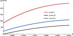
The numerical computations for position and momentum Fisher information for the three different values of α=0.1, 0.12 and 0.13 give perfect results for values of variation parameter B, because it is expected that ${I}_{r}.{I}_{p}\geqslant 36.0$ which is shown in tables 1, 2 and 3. The computation of various expectation values for different values of α also gave a good result, which is in agreement with existing literature. Here, it is expected that the Heinsenberg uncertainty relation of the product of position and momentum entropies should be given as as ${\rm{\Delta }}(r){\rm{\Delta }}(p)\geqslant \tfrac{{\hslash }}{2\pi }$ such that the squeeze state of ${\rm{\Delta }}{(r)}^{2}{\rm{\Delta }}{(p)}^{2}$ should be a minimum of 0.250 00. Tables 4, 5 and 6 gives the various expectation values for different values of α and their corresponding squeeze state. This table is in agreement with existing literature with a squeeze state value of more than 0.250 00. The expectation values of $\langle r\rangle $, $\langle {r}^{2}\rangle $ decrease with an increase in the variation parameter (B), while $\langle {p}^{2}\rangle $ and Δ (p) increase with an increase in the variation parameter (B) for α = 0.1, 0.12, and 0.13, respectively, as shown in tables 4, 5 and 6. The graph of position entropy in figure 2 for different values of α increases exponentially. However, the graph of momentum entropy as presented in figure 3 shows a clear distinction and quantisation of momentum theory for different values of α. Figure 4 is the graph of the squeeze state which is the product of position and momentum entropy with variation parameter (B) for different values of α. This graph gives a perfect curve with distinct quantisation for different values of α.

Figure 2. Fisher Position entropy for n = 0. |

Figure 3. Fisher momentum entropy for n = 0. |
Figure 4. The product of position and momentum entropy for n = 0. |
Table 1. Numerical results for Fisher information for n = 0, with various values of B, with A = 0.5 eV for the noncentral potential (NCP) for α = 0.1. |
| B | Ir | Ip | ${I}_{r}{I}_{p}\geqslant 36.0$ | min(${I}_{r}{I}_{p}$) |
|---|---|---|---|---|
| 0.001 | 0.96355 | 97.0367 | 93.4997 | 36.0 |
| 0.002 | 1.01546 | 96.2569 | 97.7455 | 36.0 |
| 0.003 | 1.06619 | 95.4925 | 101.814 | 36.0 |
| 0.004 | 1.11572 | 94.7429 | 105.707 | 36.0 |
| 0.005 | 1.16403 | 94.0077 | 109.428 | 36.0 |
| 0.006 | 1.21111 | 93.2865 | 112.981 | 36.0 |
| 0.007 | 1.25695 | 92.5789 | 116.367 | 36.0 |
| 0.008 | 1.30155 | 91.8843 | 119.592 | 36.0 |
| 0.009 | 1.34489 | 91.2025 | 122.657 | 36.0 |
| 0.010 | 1.38696 | 90.5330 | 125.566 | 36.0 |
| 0.011 | 1.46732 | 89.8755 | 128.322 | 36.0 |
| 0.012 | 1.42777 | 89.2295 | 130.928 | 36.0 |
| 0.013 | 1.50559 | 88.5949 | 133.387 | 36.0 |
| 0.014 | 1.54259 | 87.9711 | 135.703 | 36.0 |
| 0.015 | 1.57832 | 87.3580 | 137.879 | 36.0 |
| 0.016 | 1.61279 | 86.7553 | 139.918 | 36.0 |
| 0.017 | 1.64598 | 86.1625 | 141.822 | 36.0 |
| 0.018 | 1.67791 | 85.5795 | 143.595 | 36.0 |
| 0.019 | 1.70858 | 85.0061 | 145.240 | 36.0 |
| 0.020 | 1.73800 | 84.4418 | 146.760 | 36.0 |
| 0.021 | 1.76617 | 83.8865 | 148.157 | 36.0 |
| 0.022 | 1.79309 | 83.3400 | 149.436 | 36.0 |
| 0.023 | 1.81877 | 82.8020 | 150.598 | 36.0 |
| 0.024 | 1.84322 | 82.2723 | 151.646 | 36.0 |
| 0.025 | 1.86645 | 81.7507 | 152.584 | 36.0 |
| 0.026 | 1.86647 | 81.2369 | 153.413 | 36.0 |
| 0.027 | 1.90928 | 80.7309 | 154.138 | 36.0 |
| 0.028 | 1.92889 | 80.2323 | 154.759 | 36.0 |
| 0.029 | 1.94732 | 79.7410 | 155.281 | 36.0 |
| 0.030 | 1.96456 | 79.2569 | 155.705 | 36.0 |
Table 2. Numerical results for Fisher information for n = 0, with various values of B, with A = 0.5 eV for the noncentral potential (NCP) for α = 0.12. |
| B | Ir | Ip | ${I}_{r}{I}_{p}\geqslant 36.0$ | min(${I}_{r}{I}_{p}$) |
|---|---|---|---|---|
| 0.001 | 1.04867 | 64.3148 | 67.4451 | 36.0 |
| 0.002 | 1.09086 | 63.8761 | 69.6802 | 36.0 |
| 0.003 | 1.13221 | 63.4448 | 71.8329 | 36.0 |
| 0.004 | 1.17271 | 63.0204 | 73.9046 | 36.0 |
| 0.005 | 1.21235 | 62.6029 | 75.8964 | 36.0 |
| 0.006 | 1.25112 | 62.1922 | 77.8097 | 36.0 |
| 0.007 | 1.28902 | 61.7879 | 79.6457 | 36.0 |
| 0.008 | 1.32604 | 61.3899 | 81.4057 | 36.0 |
| 0.009 | 1.36219 | 60.9981 | 83.0911 | 36.0 |
| 0.010 | 1.39746 | 60.6124 | 84.7031 | 36.0 |
| 0.011 | 1.43183 | 60.2324 | 86.2429 | 36.0 |
| 0.012 | 1.46533 | 59.8582 | 87.7119 | 36.0 |
| 0.013 | 1.49793 | 59.4896 | 89.1114 | 36.0 |
| 0.014 | 1.52965 | 59.1264 | 90.4427 | 36.0 |
| 0.015 | 1.56048 | 58.7685 | 91.7069 | 36.0 |
| 0.016 | 1.59042 | 58.4158 | 92.9054 | 36.0 |
| 0.017 | 1.61947 | 58.0681 | 94.0393 | 36.0 |
| 0.018 | 1.64763 | 57.7253 | 95.1100 | 36.0 |
| 0.019 | 1.67491 | 57.3873 | 96.1187 | 36.0 |
| 0.020 | 1.70131 | 57.0540 | 97.0666 | 36.0 |
| 0.021 | 1.72682 | 56.7254 | 97.9548 | 36.0 |
| 0.022 | 1.75146 | 56.4012 | 98.7846 | 36.0 |
| 0.023 | 1.77523 | 56.0814 | 99.5571 | 36.0 |
| 0.024 | 1.79812 | 55.7658 | 100.274 | 36.0 |
| 0.025 | 1.82014 | 55.4545 | 100.935 | 36.0 |
| 0.026 | 1.84130 | 55.1472 | 101.543 | 36.0 |
| 0.027 | 1.86160 | 54.8440 | 102.098 | 36.0 |
| 0.028 | 1.88105 | 54.5446 | 102.601 | 36.0 |
| 0.029 | 1.89964 | 54.2491 | 103.054 | 36.0 |
| 0.030 | 1.91739 | 53.9574 | 103.458 | 36.0 |
Table 3. Numerical results for Fisher information for n = 0, with various values of B, with A = 0.5 eV for the noncentral potential (NCP) for α = 0.13. |
| B | Ir | Ip | ${I}_{r}{I}_{p}\geqslant 36.0$ | min(${I}_{r}{I}_{p}$) |
|---|---|---|---|---|
| 0.001 | 1.08189 | 53.5829 | 57.9710 | 36.0 |
| 0.002 | 1.09086 | 53.2419 | 59.6565 | 36.0 |
| 0.003 | 1.13221 | 52.9061 | 61.2833 | 36.0 |
| 0.004 | 1.17271 | 52.5754 | 62.8524 | 36.0 |
| 0.005 | 1.21235 | 52.2496 | 64.3646 | 36.0 |
| 0.006 | 1.25112 | 51.9287 | 65.8206 | 36.0 |
| 0.007 | 1.28902 | 51.6126 | 67.2214 | 36.0 |
| 0.008 | 1.32604 | 51.3010 | 68.5679 | 36.0 |
| 0.009 | 1.36219 | 50.9939 | 69.8610 | 36.0 |
| 0.010 | 1.39746 | 50.6912 | 71.1014 | 36.0 |
| 0.011 | 1.43183 | 50.3928 | 72.2901 | 36.0 |
| 0.012 | 1.46533 | 50.0986 | 73.4279 | 36.0 |
| 0.013 | 1.49793 | 49.8084 | 74.5157 | 36.0 |
| 0.014 | 1.52965 | 49.5223 | 75.5544 | 36.0 |
| 0.015 | 1.56048 | 49.2400 | 76.5447 | 36.0 |
| 0.016 | 1.59042 | 48.9616 | 77.4876 | 36.0 |
| 0.017 | 1.61947 | 48.6869 | 78.3838 | 36.0 |
| 0.018 | 1.64763 | 48.4159 | 79.2343 | 36.0 |
| 0.019 | 1.67491 | 48.1484 | 80.0398 | 36.0 |
| 0.020 | 1.70131 | 47.8843 | 80.8011 | 36.0 |
| 0.021 | 1.72682 | 47.6237 | 81.5191 | 36.0 |
| 0.022 | 1.75146 | 47.3665 | 82.1946 | 36.0 |
| 0.023 | 1.77523 | 47.1125 | 82.8283 | 36.0 |
| 0.024 | 1.79812 | 46.8617 | 83.4210 | 36.0 |
| 0.025 | 1.82014 | 46.6140 | 83.9736 | 36.0 |
| 0.026 | 1.84130 | 46.3694 | 84.4868 | 36.0 |
| 0.027 | 1.86160 | 46.1277 | 84.9613 | 36.0 |
| 0.028 | 1.88105 | 45.8890 | 85.3979 | 36.0 |
| 0.029 | 1.89964 | 45.6533 | 85.7974 | 36.0 |
| 0.030 | 1.91739 | 45.4203 | 86.1604 | 36.0 |
Table 4. Numerical results for uncertainty relation in the ground eigenstates for various values of B, with n, l = 0, A = 0.5 eV α = 0.1. |
| B | $\left\langle {r}^{2}\right\rangle $ | $\left\langle r\right\rangle $ | Δ (r) | (Δr)2 | $\left\langle {p}^{2}\right\rangle $ | Δ (p) | ${\rm{\Delta }}(r){\rm{\Delta }}(p)\geqslant \tfrac{{\hslash }}{2}$ | ${({\rm{\Delta }}r)}^{2}{({\rm{\Delta }}p)}^{2}$ | min $\left\{{({\rm{\Delta }}r)}^{2}{({\rm{\Delta }}p)}^{2}\right\}$ |
|---|---|---|---|---|---|---|---|---|---|
| 0.001 | 24.2592 | 3.40874 | 3.55523 | 2.90712 | 0.96354 | 0.490803 | 1.74492 | 3.04474 | 0.250000 |
| 0.002 | 24.0642 | 3.39462 | 3.54130 | 2.89748 | 1.01546 | 0.503851 | 1.78429 | 3.18368 | 0.250000 |
| 0.003 | 23.8731 | 3.38073 | 3.52757 | 2.88797 | 1.06619 | 0.516283 | 1.82123 | 3.31687 | 0.250000 |
| 0.004 | 23.6857 | 3.36707 | 3.51406 | 2.87857 | 1.11572 | 0.528139 | 1.85591 | 3.44440 | 0.250000 |
| 0.005 | 23.5019 | 3.35362 | 3.50074 | 2.86929 | 1.16403 | 0.539452 | 1.88848 | 3.56635 | 0.250000 |
| 0.006 | 23.3216 | 3.34038 | 3.48762 | 2.86013 | 1.21111 | 0.550253 | 1.91907 | 3.68284 | 0.250000 |
| 0.007 | 23.1447 | 3.32735 | 3.47469 | 2.85107 | 1.25695 | 0.560570 | 1.94781 | 3.79395 | 0.250000 |
| 0.008 | 22.9711 | 3.31451 | 3.46195 | 2.84213 | 1.30155 | 0.570427 | 1.97479 | 3.89979 | 0.250000 |
| 0.009 | 22.8006 | 3.30187 | 3.44939 | 2.83329 | 1.34488 | 0.579846 | 2.00011 | 4.00046 | 0.250000 |
| 0.010 | 22.6332 | 3.28941 | 3.43700 | 2.82456 | 1.38696 | 0.588847 | 2.02387 | 4.09604 | 0.250000 |
| 0.011 | 22.4689 | 3.27714 | 3.42479 | 2.81593 | 1.42777 | 0.597447 | 2.04613 | 4.18666 | 0.250000 |
| 0.012 | 22.3074 | 3.26505 | 3.41275 | 2.80740 | 1.46731 | 0.605664 | 2.06698 | 4.27240 | 0.250000 |
| 0.013 | 22.1487 | 3.25312 | 3.40087 | 2.28090 | 1.50558 | 0.613512 | 2.08647 | 4.35337 | 0.250000 |
| 0.014 | 21.9928 | 3.24137 | 3.38914 | 2.79063 | 1.54259 | 0.621005 | 2.10468 | 4.42967 | 0.250000 |
| 0.015 | 21.8395 | 3.22978 | 3.37758 | 2.78239 | 1.57832 | 0.628157 | 2.12165 | 4.50139 | 0.250000 |
| 0.016 | 21.6888 | 3.21835 | 3.36616 | 2.77424 | 1.61278 | 0.634977 | 2.13744 | 4.56864 | 0.250000 |
| 0.017 | 21.5406 | 3.20707 | 3.35495 | 2.76618 | 1.64598 | 0.641479 | 2.15209 | 4.63151 | 0.250000 |
| 0.018 | 21.3949 | 3.19595 | 3.34377 | 2.75821 | 1.67791 | 0.647671 | 2.16567 | 4.69011 | 0.250000 |
| 0.019 | 21.2515 | 3.18497 | 3.33279 | 2.75032 | 1.70858 | 0.653564 | 2.17819 | 4.74452 | 0.250000 |
| 0.020 | 21.1105 | 3.17414 | 3.32195 | 2.74252 | 1.73799 | 0.659166 | 2.18971 | 4.79485 | 0.250000 |
| 0.021 | 20.9716 | 3.16344 | 3.31123 | 2.73480 | 1.76616 | 0.664486 | 2.20027 | 4.84118 | 0.250000 |
| 0.022 | 20.8350 | 3.15288 | 3.30066 | 2.72716 | 1.79308 | 0.669531 | 2.20989 | 4.88362 | 0.250000 |
| 0.023 | 20.7005 | 3.14246 | 3.29020 | 2.71960 | 1.81877 | 0.674309 | 2.21861 | 4.92225 | 0.250000 |
| 0.024 | 20.5681 | 3.13217 | 3.27987 | 2.71212 | 1.84322 | 0.678827 | 2.22647 | 4.95716 | 0.250000 |
| 0.025 | 20.4377 | 3.12200 | 3.26967 | 2.70472 | 1.86645 | 0.683091 | 2.23348 | 4.98845 | 0.250000 |
| 0.026 | 20.3092 | 3.11196 | 3.25958 | 2.69739 | 1.88846 | 0.687108 | 2.23969 | 5.01621 | 0.250000 |
| 0.027 | 20.1827 | 3.10204 | 3.24962 | 2.69013 | 1.90927 | 0.690883 | 2.24511 | 5.04052 | 0.250000 |
| 0.028 | 20.0581 | 3.09224 | 3.23976 | 2.68295 | 1.92889 | 0.694423 | 2.24977 | 5.06146 | 0.250000 |
| 0.029 | 19.9353 | 3.08256 | 3.23003 | 2.67584 | 1.94732 | 0.697731 | 2.25369 | 5.07913 | 0.250000 |
| 0.030 | 19.8142 | 3.07299 | 3.22039 | 2.66879 | 1.96456 | 0.700815 | 2.25690 | 5.09361 | 0.250000 |
Table 5. Numerical results for uncertainty relation in the ground eigenstates for various values of B, with n, l = 0, A = 0.5 eV α = 0.12. |
| B | $\left\langle {r}^{2}\right\rangle $ | $\left\langle r\right\rangle $ | Δ (r) | (Δr)2 | $\left\langle {p}^{2}\right\rangle $ | Δ (p) | ${\rm{\Delta }}(r){\rm{\Delta }}(p)\geqslant \tfrac{{\hslash }}{2}$ | (Δr)2 (Δp)2 | min $\left\{{({\rm{\Delta }}r)}^{2}{({\rm{\Delta }}p)}^{2}\right\}$ |
|---|---|---|---|---|---|---|---|---|---|
| 0.001 | 16.0787 | 2.76177 | 2.90712 | 8.45134 | 0.262168 | 0.512023 | 1.48851 | 2.21567 | 0.250000 |
| 0.002 | 15.9690 | 2.75202 | 2.89748 | 8.39540 | 0.272716 | 0.522222 | 1.51313 | 2.28956 | 0.250000 |
| 0.003 | 15.7551 | 2.74242 | 2.88797 | 8.34035 | 0.283053 | 0.532027 | 1.53648 | 2.36076 | 0.250000 |
| 0.004 | 15.6507 | 2.73294 | 2.87857 | 8.28616 | 0.293177 | 0.541458 | 1.55863 | 2.42931 | 0.250000 |
| 0.005 | 15.6507 | 2.72358 | 2.86929 | 8.23283 | 0.303086 | 0.550532 | 1.57964 | 2.49526 | 0.250000 |
| 0.006 | 15.5480 | 2.71435 | 2.86013 | 8.18032 | 0.312779 | 0.559266 | 1.59957 | 2.55864 | 0.250000 |
| 0.007 | 15.4477 | 2.70524 | 2.85107 | 8.12862 | 0.322255 | 0.567674 | 1.61848 | 2.61948 | 0.250000 |
| 0.008 | 15.3475 | 2.69625 | 2.84213 | 8.07770 | 0.331511 | 0.575769 | 1.63641 | 2.67785 | 0.250000 |
| 0.009 | 15.2495 | 2.68737 | 2.83329 | 8.02755 | 0.340548 | 0.583564 | 1.65341 | 2.73376 | 0.250000 |
| 0.010 | 15.1531 | 2.67861 | 2.82456 | 7.97815 | 0.349364 | 0.591070 | 1.66951 | 2.78728 | 0.250000 |
| 0.011 | 15.1531 | 2.66995 | 2.81593 | 7.92947 | 0.357959 | 0.598296 | 1.68476 | 2.83842 | 0.250000 |
| 0.012 | 14.9646 | 2.66140 | 2.81593 | 7.92947 | 0.366332 | 0.605253 | 1.69919 | 2.88725 | 0.250000 |
| 0.013 | 12.2407 | 2.65296 | 2.81593 | 5.20251 | 0.374483 | 0.611950 | 1.39580 | 1.94825 | 0.250000 |
| 0.014 | 14.7816 | 2.64461 | 2.79063 | 7.78763 | 0.382412 | 0.618395 | 1.72571 | 2.97809 | 0.250000 |
| 0.015 | 14.6921 | 2.63637 | 2.78239 | 7.74170 | 0.390119 | 0.624595 | 1.73787 | 3.02019 | 0.250000 |
| 0.016 | 14.6039 | 2.62822 | 2.77423 | 7.69641 | 0.397604 | 0.630558 | 1.74932 | 3.06012 | 0.250000 |
| 0.017 | 14.5176 | 2.62017 | 2.76617 | 7.65175 | 0.404867 | 0.636291 | 1.76010 | 3.09794 | 0.250000 |
| 0.018 | 14.4313 | 2.61221 | 2.75821 | 7.60771 | 0.411908 | 0.641800 | 1.77022 | 3.13367 | 0.250000 |
| 0.019 | 14.3468 | 2.60434 | 2.75032 | 7.56426 | 0.418728 | 0.647091 | 1.77971 | 3.16737 | 0.250000 |
| 0.020 | 14.2635 | 2.59656 | 2.74252 | 7.52140 | 0.425327 | 0.652171 | 1.78859 | 3.19906 | 0.250000 |
| 0.021 | 14.1813 | 2.58887 | 2.73479 | 7.47912 | 0.431706 | 0.657043 | 1.79688 | 3.22878 | 0.250000 |
| 0.022 | 14.1003 | 2.58126 | 2.72715 | 7.43740 | 0.437866 | 0.661714 | 1.80460 | 3.25658 | 0.250000 |
| 0.023 | 14.0203 | 2.57374 | 2.71960 | 7.39623 | 0.443806 | 0.666187 | 1.81177 | 3.28249 | 0.250000 |
| 0.024 | 13.9415 | 2.56629 | 2.71212 | 7.35560 | 0.449529 | 0.670469 | 1.81839 | 3.30656 | 0.250000 |
| 0.025 | 13.8636 | 2.55893 | 2.70471 | 7.31549 | 0.455035 | 0.674563 | 1.82450 | 3.32881 | 0.250000 |
| 0.026 | 13.7868 | 2.55165 | 2.69738 | 7.27590 | 0.460325 | 0.678472 | 1.83010 | 3.34928 | 0.250000 |
| 0.027 | 13.7110 | 2.54444 | 2.69013 | 7.23681 | 0.465401 | 0.682202 | 1.83522 | 3.36801 | 0.250000 |
| 0.028 | 13.6362 | 2.53731 | 2.68294 | 7.19821 | 0.470262 | 0.685756 | 1.83985 | 3.38505 | 0.250000 |
| 0.029 | 13.5623 | 2.53025 | 2.67583 | 7.16010 | 0.474911 | 0.689137 | 1.84402 | 3.40041 | 0.250000 |
| 0.030 | 13.4893 | 2.52327 | 2.66879 | 7.12245 | 0.479349 | 0.692350 | 1.84774 | 3.41414 | 0.250000 |
Table 6. Numerical results for uncertainty relation in the ground eigenstates for various values of B, with n, l = 0, A = 0.5 eV α = 0.13. |
| B | $\left\langle {r}^{2}\right\rangle $ | $\left\langle r\right\rangle $ | Δ (r) | (Δr)2 | $\left\langle {p}^{2}\right\rangle $ | Δ (p) | ${\rm{\Delta }}(r){\rm{\Delta }}(p)\geqslant \tfrac{{\hslash }}{2}$ | (Δr)2 (Δp)2 | min $\left\{{({\rm{\Delta }}r)}^{2}{({\rm{\Delta }}p)}^{2}\right\}$ |
|---|---|---|---|---|---|---|---|---|---|
| 0.001 | 13.3957 | 2.51467 | 2.65936 | 7.07218 | 0.270473 | 0.520070 | 1.38305 | 1.91283 | 0.250000 |
| 0.002 | 13.3105 | 2.50638 | 2.65114 | 7.02855 | 0.280120 | 0.529264 | 1.40315 | 1.96884 | 0.250000 |
| 0.003 | 13.2265 | 2.49819 | 2.64302 | 6.98557 | 0.283053 | 0.538131 | 1.42229 | 2.02292 | 0.250000 |
| 0.004 | 13.1438 | 2.49011 | 2.63500 | 6.94322 | 0.298868 | 0.546688 | 1.44052 | 2.07511 | 0.250000 |
| 0.005 | 13.0624 | 2.48212 | 2.62707 | 6.90148 | 0.307966 | 0.554947 | 1.45788 | 2.12543 | 0.250000 |
| 0.006 | 12.9822 | 2.47423 | 2.61923 | 6.86035 | 0.316879 | 0.562920 | 1.47442 | 2.17390 | 0.250000 |
| 0.007 | 12.9031 | 2.46644 | 2.61147 | 6.81979 | 0.325606 | 0.570619 | 1.49016 | 2.22057 | 0.250000 |
| 0.008 | 12.8252 | 2.45875 | 2.60381 | 6.77981 | 0.334145 | 0.578053 | 1.50514 | 2.26544 | 0.250000 |
| 0.009 | 12.7485 | 2.45114 | 2.59623 | 6.74039 | 0.342497 | 0.585232 | 1.51940 | 2.30856 | 0.250000 |
| 0.010 | 12.6728 | 2.44362 | 2.58873 | 6.70151 | 0.350660 | 0.592165 | 1.53295 | 2.34995 | 0.250000 |
| 0.011 | 12.5982 | 2.43619 | 2.58131 | 6.66317 | 0.358633 | 0.598860 | 1.54584 | 2.38963 | 0.250000 |
| 0.012 | 12.5246 | 2.42885 | 2.57398 | 6.62535 | 0.366417 | 0.605324 | 1.55809 | 2.42764 | 0.250000 |
| 0.013 | 12.4521 | 2.42158 | 2.56672 | 6.58804 | 0.374012 | 0.611565 | 1.56971 | 2.46400 | 0.250000 |
| 0.014 | 12.3806 | 2.41441 | 2.55954 | 6.55122 | 0.381416 | 0.617589 | 1.58074 | 2.49874 | 0.250000 |
| 0.015 | 12.3100 | 2.40731 | 2.55243 | 6.51489 | 0.388630 | 0.623402 | 1.59119 | 2.53188 | 0.250000 |
| 0.016 | 12.2404 | 2.40028 | 2.54540 | 6.47904 | 0.395655 | 0.629011 | 1.60108 | 2.56346 | 0.250000 |
| 0.017 | 12.1717 | 2.39334 | 2.53844 | 6.44365 | 0.402489 | 0.634420 | 1.61044 | 2.59350 | 0.250000 |
| 0.018 | 12.1040 | 2.38647 | 2.53155 | 6.40872 | 0.409134 | 0.639636 | 1.61927 | 2.62203 | 0.250000 |
| 0.019 | 12.0371 | 2.37967 | 2.52473 | 6.37424 | 0.415589 | 0.644662 | 1.62760 | 2.64907 | 0.250000 |
| 0.020 | 11.9711 | 2.37295 | 2.51797 | 6.34019 | 0.421856 | 0.649504 | 1.63543 | 2.67465 | 0.250000 |
| 0.021 | 11.9059 | 2.36630 | 2.51129 | 6.30657 | 0.427933 | 0.654166 | 1.64280 | 2.69879 | 0.250000 |
| 0.022 | 11.8416 | 2.35971 | 2.50467 | 6.27337 | 0.433822 | 0.658652 | 1.64971 | 2.72153 | 0.250000 |
| 0.023 | 11.7781 | 2.35320 | 2.49812 | 6.24058 | 0.439524 | 0.662966 | 1.65617 | 2.74289 | 0.250000 |
| 0.024 | 11.7154 | 2.34675 | 2.49162 | 6.20819 | 0.445039 | 0.667112 | 1.66219 | 2.76289 | 0.250000 |
| 0.025 | 11.6535 | 2.34036 | 2.48519 | 6.17619 | 0.450367 | 0.671094 | 1.66780 | 2.78155 | 0.250000 |
| 0.026 | 11.5923 | 2.33404 | 2.47883 | 6.14458 | 0.455510 | 0.674915 | 1.67300 | 2.79892 | 0.250000 |
| 0.027 | 11.5319 | 2.32779 | 2.47252 | 6.11335 | 0.460467 | 0.678577 | 1.67780 | 2.8150 | 0.250000 |
| 0.028 | 11.4723 | 2.32159 | 2.46627 | 6.08248 | 0.465241 | 0.682086 | 1.68221 | 2.82982 | 0.250000 |
| 0.029 | 11.4133 | 2.31546 | 2.46008 | 6.05198 | 0.469831 | 0.685442 | 1.68624 | 2.84341 | 0.250000 |
| 0.030 | 11.3551 | 2.30938 | 2.45394 | 6.02184 | 0.474240 | 0.688651 | 1.68991 | 2.85579 | 0.250000 |
8. Conclusion
In this work, we develop a class of noncentral potential (noncentral inversely quadratic plus exponential Mie-type potential) to investigate the quantum information of Fisher and Shannon entropies in a Schrödinger equation. We obtained the normalised wave function and energy-eigen equations by solving the radial solution of the Schrödinger equation via the Nikiforov–Uvarov method. We analytically obtain position and momentum space for both Fisher and Shannon entropies and calculation were carried out with ground state wave function where the principal quantum number n and orbital quantum number l equals zero. The numerical computations were only carried out for Fisher information in position and momentum space, since that of Shannon was a great deal more complicated due to the nature of the potential. All computations were carried out for α = 0.1, 0.12 and 0.13 because these are the only set of values that give the expected result. However, the wave function plots and probability density curves were plotted only for α = 0.1 because this is the best value of α that gave the best plot. The normalisation constants were obtained using confluent hypergeometric functions with the help of Mathematica. The expectation values obtained with respect to position entropy decreases with an increase in variation parameter (B), whereas that of momentum increases with an increase in this parameter. All the numerical results obtained are in agreement with existing literature, including Heinsenberg uncertainties for position and momentum. The study of these entropies is very significant in terms of their potential applications in signal processing and examining the electronic structures of atoms.