


1. Introduction
As we know, the model of many natural phenomena and differential equations in science and engineering are nonlinear, and it is very important to obtain analytically or numerically accurate solutions. In order to achieve this goal, various methods have been developed for linear and nonlinear equations such as: the Exp-function method [1], the homotopy analysis method [2], the homotopy perturbation method [3], the (G’/G)-expansion method [4], the improved $\tan (\phi /2)$ -expansion method [5, 6], Hirota’s bilinear method [7–19], He’s variational principle [20, 21], the binary Darboux transformation [22], the Lie group analysis [23, 24], the Bäcklund transformation method [25], and the multiple Exp-function method [26, 27]. Moreover, many powerful methods have been used to investigate the new properties of mathematical models symbolizing serious real world problems [28–30].
Bogoyavlenski introduced a model equation to describe nonisospectral scattering problems [31], specifically the (2+1)-dimensional Bogoyavlenski equation: $ \begin{eqnarray}4{{\rm{\Psi }}}_{t}+{{\rm{\Psi }}}_{{xxy}}-4{{\rm{\Psi }}}^{2}{{\rm{\Psi }}}_{y}-4{{\rm{\Psi }}}_{x}{\rm{\Phi }}=0,\end{eqnarray}$
$ \begin{eqnarray*}{\rm{\Psi }}{{\rm{\Psi }}}_{y}={{\rm{\Phi }}}_{x}.\end{eqnarray*}$ Kudryashov and Pickering [32] proposed the above equation as a member of a (2 + 1) Schwarzian breaking soliton hierarchy. Clarkson and co-authors [33] investigated equation (1.1 ) as part of a group of equations associated with nonisospectral scattering problems. Estevez and Prada [34] presented a generalization of the sine-Gordon equation possessing the Painleve feature. Zhran and Khater [35] examined the Bogoyavlenskii equation utilizing the modified extended tanh-function method. The authors of [36] showed that the above equation is an as-modified version of the following nonlinear equation: $ \begin{eqnarray}4{{\rm{\Psi }}}_{{xt}}+8{{\rm{\Psi }}}_{x}{{\rm{\Psi }}}_{{xy}}+4{{\rm{\Psi }}}_{y}{{\rm{\Psi }}}_{{xx}}+{{\rm{\Psi }}}_{{xxxy}}=0,\end{eqnarray}$ this is known as the breaking soliton equation. Equation (1.2 ) is also a specific version of a form of Bogoyavlensky–Konopelchenko (BK) equation, given as $ \begin{eqnarray}\begin{array}{l}a{{\rm{\Psi }}}_{{xt}}+b{{\rm{\Psi }}}_{{xxxx}}+c{{\rm{\Psi }}}_{{xxy}}+d{{\rm{\Psi }}}_{x}{{\rm{\Psi }}}_{{xx}}\\ \qquad +\,e{{\rm{\Psi }}}_{x}{{\rm{\Psi }}}_{{xy}}+k{{\rm{\Psi }}}_{{xx}}{{\rm{\Psi }}}_{y}=0.\end{array}\end{eqnarray}$ The BK equation defines the (2+1)-dimensional interaction of a Riemann wave propagation along the y-axis with a long wave along the x-axis, and is also a two-dimensional generalization of the well known Korteweg-de Vries equation [37, 38]. This study is aimed at investigating the following generalized BK equation [39]: $ \begin{eqnarray}\begin{array}{l}{{\rm{\Psi }}}_{t}+\alpha (6{\rm{\Psi }}{{\rm{\Psi }}}_{x}+{{\rm{\Psi }}}_{{xxx}})+\beta ({{\rm{\Psi }}}_{{xxy}}+3{\rm{\Psi }}{{\rm{\Psi }}}_{y}+3{{\rm{\Psi }}}_{x}{{\rm{\Phi }}}_{y})\\ \,+\,{\gamma }_{1}{{\rm{\Psi }}}_{x}+{\gamma }_{2}{{\rm{\Psi }}}_{y}+{\gamma }_{3}{{\rm{\Phi }}}_{{yy}}=0,\end{array}\end{eqnarray}$ in which Φx = ψ, and α, β, γ1, γ2, and γ3 are determined values. Equation (1.4 ) can be written as $ \begin{eqnarray}\begin{array}{l}{{\rm{\Phi }}}_{{xt}}+\alpha (6{{\rm{\Phi }}}_{x}{{\rm{\Phi }}}_{{xx}}+{{\rm{\Phi }}}_{{xxxx}})+\beta ({{\rm{\Phi }}}_{{xxxy}}+3{{\rm{\Phi }}}_{x}{{\rm{\Phi }}}_{{xy}}+3{{\rm{\Phi }}}_{{xx}}{{\rm{\Phi }}}_{{xy}})\\ \,+\,{\gamma }_{1}{{\rm{\Phi }}}_{{xx}}+{\gamma }_{2}{{\rm{\Phi }}}_{{xy}}+{\gamma }_{3}{{\rm{\Phi }}}_{{yy}}=0,\end{array}\end{eqnarray}$ by applying the bilinear transformation ${\rm{\Psi }}=2{(\mathrm{ln}f)}_{{xx}}$ and ${\rm{\Phi }}=2{(\mathrm{ln}f)}_{x}$ , the equation (1.5 ) transforms to the bilinear form as follows: $ \begin{eqnarray}\begin{array}{l}\left(\alpha {D}_{x}^{4}+\beta {D}_{x}^{3}{D}_{y}+{D}_{t}{D}_{x}+{\gamma }_{1}{D}_{x}^{2}\right.\\ \,\left.+\,{\gamma }_{2}{D}_{x}{D}_{y}+{\gamma }_{3}{D}_{y}^{2}\right){\mathfrak{f}}.{\mathfrak{f}}=0,\end{array}\end{eqnarray}$
$ \begin{eqnarray*}\begin{array}{l}{D}_{x}^{4}{\mathfrak{f}}.{\mathfrak{f}}=2({{\mathfrak{ff}}}_{{xxxx}}-4{{\mathfrak{f}}}_{x}{{\mathfrak{f}}}_{{xxx}}+3{{\mathfrak{f}}}_{{xx}}^{2}),\\ {D}_{x}^{3}{D}_{y}{\mathfrak{f}}.{\mathfrak{f}}=2({{\mathfrak{ff}}}_{{xxxy}}-{{\mathfrak{f}}}_{y}{{\mathfrak{f}}}_{{xxx}}-3{{\mathfrak{f}}}_{x}{{\mathfrak{f}}}_{{xxy}}+3{{\mathfrak{f}}}_{{xx}}{{\mathfrak{f}}}_{{xy}}),\end{array}\end{eqnarray*}$
$ \begin{eqnarray*}\begin{array}{l}{D}_{x}^{2}{\mathfrak{f}}.{\mathfrak{f}}=2({{\mathfrak{ff}}}_{{xx}}-{{\mathfrak{f}}}_{x}^{2}),\ \ \ {D}_{x}{D}_{t}{\mathfrak{f}}.{\mathfrak{f}}=2({{\mathfrak{ff}}}_{{xt}}-{{\mathfrak{f}}}_{x}{{\mathfrak{f}}}_{t}),\\ {D}_{x}{D}_{y}{\mathfrak{f}}.{\mathfrak{f}}=2({{\mathfrak{ff}}}_{{xy}}-{{\mathfrak{f}}}_{x}{{\mathfrak{f}}}_{y}),\ \ {D}_{y}^{2}{\mathfrak{f}}.{\mathfrak{f}}=2({{\mathfrak{ff}}}_{{yy}}-{{\mathfrak{f}}}_{y}^{2}).\end{array}\end{eqnarray*}$
Various research models already exist relating to lump solutions for the (2+1)-dimensional nonlinear equation. Liu and co-workers employed the Hirota bilinear method to obtain an N-soliton solution for the (3+1)-dimensional generalized KP equation [40]. The same group also constructed an N-soliton solution for the(2+1)-dimensional generalized Hirota-Satsuma-Ito equation [41]. Localized nonlinear matter waves in two-component Bose-Einstein condensates with time- and space-modulated nonlinearities [42], and in a rotating Bose-Einstein condensate with spatiotemporally modulated interaction [43] have been investigated both analytically and numerically. With regard to the integrable coupled nonlinear Schrödinger system, N-soliton solutions within this system were obtained, and the collision dynamics between two solitons was also analyzed via the Riemann-Hilbert method by Wang and co-authors in [44].
Various research models already exist relating to lump solutions for the (2+1)-dimensional nonlinear equation. Liu and co-workers employed the Hirota bilinear method to obtain an N-soliton solution for the (3+1)-dimensional generalized KP equation [40]. The same group also constructed an N-soliton solution for the(2+1)-dimensional generalized Hirota-Satsuma-Ito equation [41]. Localized nonlinear matter waves in two-component Bose-Einstein condensates with time- and space-modulated nonlinearities [42], and in a rotating Bose-Einstein condensate with spatiotemporally modulated interaction [43] have been investigated both analytically and numerically. With regard to the integrable coupled nonlinear Schrödinger system, N-soliton solutions within this system were obtained, and the collision dynamics between two solitons was also analyzed via the Riemann-Hilbert method by Wang and co-authors in [44].
Currently, nonlinear differential equations represent a significant opportunity for researchers to define tangible incidents. This has driven mathematicians and scientists to examine a wide variety of soliton solutions. As a result, in the past few years a growing number of effective and realistic methods have been initiated and dilated to extract closed form solutions to NLDEs. Among these, the semi-inverse principle method is one of the more powerful methods to be examined, in studies relating to the buckling analysis of circular cylinders [45], one-dimensional compressible flow in a microgravity space [46], the generalized KdV-Burgers equation with fractal derivatives [47], and the thin film equation [48]. In addition, it would be beneficial to researchers to consider recent studies on the variational approach to nonlinear oscillators, as investigated by authors such as Liu [49], Nawaz, and co-workers [50], He [51, 52], and Kovacic, Rakaric, and Cveticanin [53]. Finally, any review of the above methods should include two-scale fractal calculus, a hot topic in mathematics and physics, as demonstrated in the valuable works [54, 55].
In this paper, we will study the multiple lump soliton to determine multiple soliton solutions. The multiple lump method has been utilized by researchers for a variety of applications requiring nonlinear equations, including: the construction of rogue waves with a controllable center in nonlinear systems [56], the (3+1)-dimensional Hirota bilinear equation [57], the generalized (3+1)-dimensional KP equation [58], and the Boussinesq equation [59].
The remainder of this paper is structured as follows: the multiple lump scheme is summarized in section 2 . In section 3 , the generalized BK equation is used to investigate first-order, second-order, and third-order wave solutions. SIVP will also be examined in section 4 . In the last section, the conclusions are presented.
2. Multiple lump solution method
Step 1. Take the following NLPDE $ \begin{eqnarray}{ \mathcal N }(x,y,t,{\rm{\Psi }},{{\rm{\Psi }}}_{x},{{\rm{\Psi }}}_{y},{{\rm{\Psi }}}_{t},{{\rm{\Psi }}}_{{xx}},{{\rm{\Psi }}}_{{xy}},{{\rm{\Psi }}}_{{tt}},\ldots )=0.\end{eqnarray}$ We commence a Painlevè analysis, using the following transformation $ \begin{eqnarray}{\rm{\Psi }}={\mathfrak{T}}(f),\end{eqnarray}$ based on the dependant variable function f.
Step 2. By means of transformation (2.2 ), the nonlinear equation (2.1 ) can be written in terms of the following Hirota’s bilinear form: $ \begin{eqnarray}{\mathfrak{G}}({D}_{\xi },{D}_{y};f)=0,\end{eqnarray}$ where $\xi =x-{ct}$ and c is a real parameter. Moreover, the D-operator [22] is given as follows: $ \begin{eqnarray}\prod _{i=1}^{2}{D}_{{\jmath}_{i}}^{{\beta }_{i}}f.g={\left.\prod _{i=1}^{2}{\left(\displaystyle \frac{\partial }{\partial {\jmath}_{i}}-\displaystyle \frac{\partial }{\partial {\jmath}_{i}^{{\prime} }}\right)}^{{\beta }_{i}}f(\jmath)g(\jmath^{\prime} )\right|}_{\jmath^{\prime} =\jmath},\end{eqnarray}$ where the vectors $\jmath=({\jmath}_{1},{\jmath}_{2},{\jmath}_{3})=(x,y,t)$ , $\jmath^{\prime} =({\jmath}_{1}^{{\prime} },{\jmath}_{2}^{{\prime} },{\jmath}_{3}^{{\prime} })=(x^{\prime} ,y^{\prime} ,t^{\prime} )$ , and β1, β2, β3 are arbitrary nonnegative integers.
Step 3. Let $ \begin{eqnarray}\begin{array}{rcl}{\mathfrak{f}} & = & {\mathfrak{f}}(\xi ,y;\theta ,\delta )\\ & = & {\chi }_{n+1}(\xi ,y)+2\delta {{yp}}_{n}(\xi ,y)\\ & & +2\delta \xi {s}_{n}(\xi ,y)+({\theta }^{2}+{\delta }^{2}){\chi }_{n-1}(\xi ,y),\end{array}\end{eqnarray}$ with $ \begin{eqnarray}{\chi }_{n}(\xi ,y)=\sum _{k=0}^{\tfrac{n(n+1)}{2}}\sum _{i=0}^{k}{a}_{n(n+1)-2k,2i}{y}^{2i}{\xi }^{n(n+1)-2k},\,\end{eqnarray}$
$ \begin{eqnarray*}{p}_{n}(\xi ,y)=\sum _{k=0}^{\tfrac{n(n+1)}{2}}\sum _{i=0}^{k}{b}_{n(n+1)-2k,2i}{y}^{2i}{\xi }^{n(n+1)-2k},\,\end{eqnarray*}$
$ \begin{eqnarray*}{s}_{n}(\xi ,y)=\sum _{k=0}^{\tfrac{n(n+1)}{2}}\sum _{i=0}^{k}{c}_{n(n+1)-2k,2i}{y}^{2i}{\xi }^{n(n+1)-2k},\,\end{eqnarray*}$ ${\chi }_{0}=1,{\chi }_{1}={p}_{0}={s}_{0}=0$ ,
where${a}_{m,l},{b}_{m,l},{c}_{m,l}(m,l\,\in \{0,2,4,...,n(n+1)\})$ and θ, δ are real values. The coefficients ${a}_{m,l},{b}_{m,l},{c}_{m,l}$ can be found, and special values θ, δ are utilized to control the wave center.
where
Step 4. By inserting (2.6 ) into (2.5 ) and setting all the coefficients of the diverse powers of ${y}^{m}{\xi }^{m}$ to zero, we obtain a system of nonlinear algebra equations. Using the symbolic computation system Maple or Mathematica, solving the system gained above leads to the values of ${a}_{m,l},{b}_{m,l},{c}_{m,l}(m,l\in \{0,2,4,...,n(n+1)\})$ .
Step 5. Plugging the values of ${a}_{m,l},{b}_{m,l},{c}_{m,l}(m,l\,\in \{0,2,4,...,n(n+1)\})$ into (2.4 ) gives some rational solutions to the (2 + 1)-dimensional generalized BK equation (1.5 ), which are then utilized to search for lump solutions. This type of lump solution is localized in y and ξ.
3. Lump solutions of a (2+1)-D generalized BK equation
3.1. Set I: one-wave solution
We commence with a one-wave function based on $\xi =x-{ct}$ , whereby equation (1.5 ) is transformed as follows: $ \begin{eqnarray}\left(\alpha {D}_{\xi }^{4}+\beta {D}_{\xi }^{3}{D}_{y}+({\gamma }_{1}-c){D}_{\xi }^{2}+{\gamma }_{2}{D}_{\xi }{D}_{y}+{\gamma }_{3}{D}_{y}^{2}\right){\mathfrak{f}}.{\mathfrak{f}}=0,\end{eqnarray}$ where c is the unfound constant, and
$ \begin{eqnarray*}\begin{array}{rcl}{D}_{\xi }^{4}{\mathfrak{f}}.{\mathfrak{f}} & = & 2({{\mathfrak{ff}}}_{\xi \xi \xi \xi }-4{{\mathfrak{f}}}_{\xi }{{\mathfrak{f}}}_{\xi \xi \xi }+3{{\mathfrak{f}}}_{\xi \xi }^{2}),\\ {D}_{\xi }^{3}{D}_{y}{\mathfrak{f}}.{\mathfrak{f}} & = & 2({{\mathfrak{ff}}}_{\xi \xi \xi y}-{{\mathfrak{f}}}_{y}{{\mathfrak{f}}}_{\xi \xi \xi }-3{{\mathfrak{f}}}_{\xi }{{\mathfrak{f}}}_{\xi \xi y}+3{{\mathfrak{f}}}_{\xi \xi }{{\mathfrak{f}}}_{\xi y}),\\ {D}_{\xi }^{2}{\mathfrak{f}}.{\mathfrak{f}} & = & 2({{\mathfrak{ff}}}_{\xi \xi }-{{\mathfrak{f}}}_{\xi }^{2}),\end{array}\end{eqnarray*}$
$ \begin{eqnarray*}{D}_{\xi }{D}_{y}{\mathfrak{f}}.{\mathfrak{f}}=2({{\mathfrak{ff}}}_{\xi y}-{{\mathfrak{f}}}_{\xi }{{\mathfrak{f}}}_{y}),\ \ {D}_{y}^{2}{\mathfrak{f}}.{\mathfrak{f}}=2({{\mathfrak{ff}}}_{{yy}}-{{\mathfrak{f}}}_{y}^{2}).\end{eqnarray*}$
Based on the approach presented in section 2, as proposed by Zhaqilao [56], we are able to derive the higher order lump solutions with controllable center of the variable-coefficient (2+1)-dimensional generalized BK equation. Considering n = 0 at (2.5 ), then (2.5 ) will be given as $ \begin{eqnarray}\begin{array}{rcl}{\mathfrak{f}} & = & {{\mathfrak{f}}}_{1}(\xi ,y;\theta ,\delta )\\ & = & {\chi }_{1}(\xi ,y)+2\delta {{yp}}_{0}(\xi ,y)+2\delta \xi {s}_{0}(\xi ,y)\\ & & +({\theta }^{2}+{\delta }^{2}){\chi }_{-1}(\xi ,y)\\ & = & {a}_{2,0}{\xi }^{2}+{a}_{0,2}{y}^{2}+{a}_{0,0}.\end{array}\end{eqnarray}$ Without loss of generality, we can choose ${a}_{\mathrm{2,0}}=1$ . Plugging (3.2 ) into (3.1 ) and setting all the coefficients of the different powers of ${y}^{m}{\xi }^{m}$ to zero, we gain a system of nonlinear algebraic equations given as: $ \begin{eqnarray}\begin{array}{l}4\,{a}_{\mathrm{0,0}}{a}_{\mathrm{0,2}}{\gamma }_{3}-4\,{{ca}}_{\mathrm{0,0}}+4\,{a}_{\mathrm{0,0}}{\gamma }_{1}+24\,\alpha =0,\\ \,4\,{a}_{\mathrm{0,2}}{\gamma }_{3}+4\,c-4\,{\gamma }_{1}=0,\\ \,-4\,{a}_{0,2}^{2}{\gamma }_{3}-4\,{{ca}}_{\mathrm{0,2}}+4\,{a}_{\mathrm{0,2}}{\gamma }_{1}=0.\end{array}\end{eqnarray}$ Solving equation (3.3 ), we get $ \begin{eqnarray}{a}_{\mathrm{0,2}}=-\displaystyle \frac{c-{\gamma }_{1}}{{\gamma }_{3}},\ \ {a}_{\mathrm{0,0}}=3\,\displaystyle \frac{\alpha }{c-{\gamma }_{1}}.\end{eqnarray}$ Thus, we can obtain a solution to equation (3.2 ) as follows: $ \begin{eqnarray}{\mathfrak{f}}={{\mathfrak{f}}}_{1}(\xi ,y;\theta ,\delta )={\left(\xi -\theta \right)}^{2}-\displaystyle \frac{c-{\gamma }_{1}}{{\gamma }_{3}}{\left(y-\delta \right)}^{2}+\displaystyle \frac{3\alpha }{c-{\gamma }_{1}},\end{eqnarray}$ Assuming λ < 0, and cg(t) > 0, then the first-order lump solutions of equation (1.5 ) can be expressed as $ \begin{eqnarray}\begin{array}{rcl}{\rm{\Psi }}(\xi ,y) & = & {{\rm{\Psi }}}_{0}+\displaystyle \frac{4}{-\tfrac{{\left(y-\delta \right)}^{2}\left(c-{\gamma }_{1}\right)}{{\gamma }_{3}}+{\left(\xi -\theta \right)}^{2}+\tfrac{3\alpha }{c-{\gamma }_{1}}}\\ & & -\displaystyle \frac{2{\left(2\xi -2\theta \right)}^{2}}{{\left(-\tfrac{{\left(y-\delta \right)}^{2}\left(c-{\gamma }_{1}\right)}{{\gamma }_{3}}+{\left(\xi -\theta \right)}^{2}+\tfrac{3\alpha }{c-{\gamma }_{1}}\right)}^{2}}.\end{array}\end{eqnarray}$ It is worth mentioning that this lump has the following features: $ \begin{eqnarray}\mathop{\mathrm{lim}}\limits_{\xi \longrightarrow \pm \infty }{\rm{\Psi }}(\xi ,y)={{\rm{\Psi }}}_{0},\ \ \ \mathop{\mathrm{lim}}\limits_{y\longrightarrow \pm \infty }{\rm{\Psi }}(\xi ,y)={{\rm{\Psi }}}_{0}.\end{eqnarray}$ By selecting suitable values of parameters, the graphical representation of a periodic wave solution is presented in figures 1 and 2 which includes a 3D plot, a contour plot, a density plot, and a 2D plot where three spaces arise at spaces y = −1, y = 0, and y = 1. In figure 1 the lump has one center (δ, θ) = (2, 2), whereas in figure 2 the rogue wave has one center $(\delta ,\theta )=(-2,-2)$ . Due to our use of a simple computation, the lump has two critical points, but we investigate only one point, $({\xi }_{1},{y}_{1})=\left(\tfrac{c\theta -\theta \,{\gamma }_{1}+3\,\sqrt{\alpha \,c-\alpha \,{\gamma }_{1}}}{c-{\gamma }_{1}},\delta \right)$ . At point (ξ1, y1), the second-order derivative and Hessian matrix can be determined, as given in [60]: $ \begin{eqnarray}\left\{\begin{array}{l}{\rm{\Theta }}1={\left.\tfrac{{\partial }^{2}}{\partial {\xi }^{2}}{\rm{\Psi }}(\xi ,y)\right|}_{({\xi }_{1},{y}_{1})}=\tfrac{1}{12}\tfrac{{\left(c-{\gamma }_{1}\right)}^{2}}{{\alpha }^{2}},\\ {{\rm{\Delta }}}_{1}={\det }{\left(\begin{array}{cc}\tfrac{{\partial }^{2}}{\partial {\xi }^{2}}{\rm{\Psi }}(\xi ,y) & \tfrac{{\partial }^{2}}{\partial \xi \partial y}{\rm{\Psi }}(\xi ,y)\\ \tfrac{{\partial }^{2}}{\partial \xi \partial y}{\rm{\Psi }}(\xi ,y) & \tfrac{{\partial }^{2}}{\partial {y}^{2}}{\rm{\Psi }}(\xi ,y)\end{array}\right)}_{({\xi }_{1},{y}_{1})}=-\tfrac{\left({c}^{2}-2\,c{\gamma }_{1}+{\gamma }_{1}^{2}\right){\left(c-{\gamma }_{1}\right)}^{3}}{108\,{\alpha }^{4}{\gamma }_{3}}.\end{array}\right.\end{eqnarray}$ If $\tfrac{c-{\gamma }_{1}}{{\gamma }_{3}}\lt 0$ , and Δ1 > 0, then point (ξ1, y1) is the extreme value point. Based on the above analysis, point (ξ1, y1) is a maximum value point at which ${{\rm{\Psi }}}_{\max }$ . By using different C and λ values, the lump solution ψ(ξ, y) has one maximum value containing ${{\rm{\Psi }}}_{\max }=\tfrac{1}{6}\tfrac{6\,\alpha \,{\psi }_{0}-c+{\gamma }_{1}}{\alpha }$ .
Based on the approach presented in section 2, as proposed by Zhaqilao [56], we are able to derive the higher order lump solutions with controllable center of the variable-coefficient (2+1)-dimensional generalized BK equation. Considering n = 0 at (
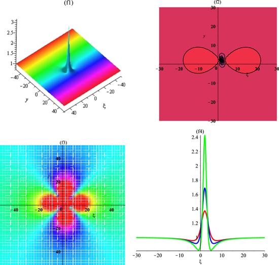
Figure 1. The one-order lump ( |
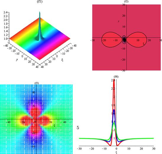
Figure 2. The one-order lump ( |
3.2. Set II: second-wave solutions
We commence with two-wave functions based on the statement in step 2 in the previous section. Here, we suppose that equation (1.5 ) has the rational function of two-wave solutions. Taking n = 1 at (2.5 ), then (2.5 ) will be expressed as $ \begin{eqnarray}\begin{array}{rcl}{\mathfrak{f}} & = & {{\mathfrak{f}}}_{2}(\xi ,y;\theta ,\delta )={\chi }_{2}(\xi ,y)+2\delta {{yp}}_{1}(\xi ,y)+2\delta \xi {s}_{1}(\xi ,y)\\ & & +({\theta }^{2}+{\delta }^{2}){\chi }_{0}(\xi ,y)={\xi }^{6}+{a}_{\mathrm{4,2}}{y}^{2}{\xi }^{4}\\ & & +{a}_{\mathrm{2,4}}{y}^{4}{\xi }^{2}+{a}_{\mathrm{0,6}}{y}^{6}\\ & & +{a}_{\mathrm{4,0}}{\xi }^{4}+{a}_{\mathrm{2,2}}{y}^{2}{\xi }^{2}+{a}_{\mathrm{0,4}}{y}^{4}+{a}_{\mathrm{2,0}}{\xi }^{2}+{a}_{\mathrm{0,2}}{y}^{2}+{a}_{\mathrm{0,0}}\\ & & +2\,\delta \,y\left({\xi }^{2}{b}_{\mathrm{2,0}}+{y}^{2}{b}_{\mathrm{0,2}}+{b}_{\mathrm{0,0}}\right)\\ & & +2\,\theta \,\xi \left({\xi }^{2}{c}_{\mathrm{2,0}}+{y}^{2}{c}_{\mathrm{0,2}}+{c}_{\mathrm{0,0}}\right)+{\delta }^{2}+{\theta }^{2}.\end{array}\end{eqnarray}$ Without loss of generality, we can choose ${a}_{\mathrm{6,0}}=1$ . Plugging (3.9 ) into (3.1 ), and setting all the coefficients of the different powers of ${y}^{m}{\xi }^{m}$ to zero, we gain a system of nonlinear algebraic equations, and by solving the related system we can express the following parameters: $ \begin{eqnarray}\begin{array}{rclcl}{a}_{\mathrm{0,0}} & = & -\displaystyle \frac{1}{3}\displaystyle \frac{-{\delta }^{2}{a}_{4,2}^{2}{b}_{2,0}^{2}{\gamma }_{3}^{3}+3\,{\delta }^{2}{a}_{4,2}^{3}{\gamma }_{3}^{3}+3\,{\theta }^{2}{a}_{4,2}^{3}{\gamma }_{3}^{3}-3\,{\theta }^{2}{a}_{\mathrm{4,2}}{c}_{0,2}^{2}{\gamma }_{3}^{3}+151875\,{\alpha }^{3}}{{a}_{4,2}^{3}{\gamma }_{3}^{3}},{a}_{\mathrm{0,2}} & = & 1425\,\displaystyle \frac{{\alpha }^{2}}{{a}_{\mathrm{4,2}}{\gamma }_{3}^{2}},\ \end{array}\end{eqnarray}$
$ \begin{eqnarray*}\begin{array}{rcl}{a}_{\mathrm{0,4}} & = & -\displaystyle \frac{17\,\alpha \,{a}_{\mathrm{4,2}}}{3\,{\gamma }_{3}},\ {a}_{\mathrm{0,6}}=\displaystyle \frac{1}{27}{a}_{4,2}^{3},\ {a}_{\mathrm{2,0}}=-1125\,\displaystyle \frac{{\alpha }^{2}}{{a}_{4,2}^{2}{\gamma }_{3}^{2}},\\ {a}_{\mathrm{2,2}} & = & -90\,\displaystyle \frac{\alpha }{{\gamma }_{3}},\ {a}_{\mathrm{2,4}}=\displaystyle \frac{1}{3}{a}_{4,2}^{2},\ {a}_{\mathrm{4,0}}=-75\,\displaystyle \frac{\alpha }{{a}_{\mathrm{4,2}}{\gamma }_{3}},\end{array}\end{eqnarray*}$
$ \begin{eqnarray*}\begin{array}{rcl}{a}_{\mathrm{4,2}} & = & -3\,\displaystyle \frac{c-{\gamma }_{1}}{{\gamma }_{3}},\ {b}_{\mathrm{0,0}}=-5\,\displaystyle \frac{{b}_{\mathrm{2,0}}\alpha }{{a}_{\mathrm{4,2}}{\gamma }_{3}},\ {b}_{\mathrm{0,2}}=-\displaystyle \frac{1}{9}{a}_{\mathrm{4,2}}{b}_{\mathrm{2,0}},\\ {b}_{\mathrm{2,0}} & = & {b}_{\mathrm{2,0}},\ {c}_{\mathrm{0,0}}=-3\,\displaystyle \frac{{c}_{\mathrm{0,2}}\alpha }{{a}_{4,2}^{2}{\gamma }_{3}},\ {c}_{\mathrm{0,2}}={c}_{\mathrm{0,2}},\ {c}_{\mathrm{2,0}}=-\displaystyle \frac{{c}_{\mathrm{0,2}}}{{a}_{\mathrm{4,2}}},\end{array}\end{eqnarray*}$
in which${b}_{\mathrm{2,0}}$ and ${c}_{\mathrm{0,2}}$ are arbitrary values. Thus, the second-order lump solutions of equation (1.5 ) can be obtained by $ \begin{eqnarray}{\rm{\Psi }}(\xi ,y)=2{\left(\mathrm{ln}{{\mathfrak{f}}}_{2}(\xi ,y;\theta ,\delta \right)}_{\xi \xi },\end{eqnarray}$ where ${{\mathfrak{f}}}_{2}(\xi ,y;\theta ,\delta )$ is given in equation (3.9 ). It is worth mentioning that this lump displays the following features: $ \begin{eqnarray}\mathop{\mathrm{lim}}\limits_{\xi \longrightarrow \pm \infty }{\rm{\Psi }}(\xi ,y)={{\rm{\Psi }}}_{0},\ \ \ \mathop{\mathrm{lim}}\limits_{y\longrightarrow \pm \infty }{\rm{\Psi }}(\xi ,y)={{\rm{\Psi }}}_{0}.\end{eqnarray}$ By selecting suitable values of parameters, the graphical representation of periodic wave solution is presented in figures 3 and 4 including 3D plot, contour plot, density plot, and 2D plot where three spaces arise at spaces $y=-1$ , y = 0, and y = 1. In figure 3 the rogue wave has one center (δ, θ) = (2, 3), whereas in figure 4 the lump has one center $(\delta ,\theta )=(-2,-3)$ .
in which
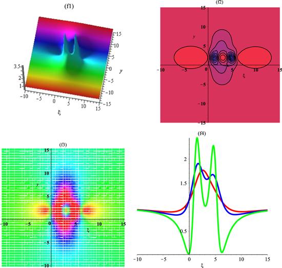
Figure 3. The second-order lump ( |
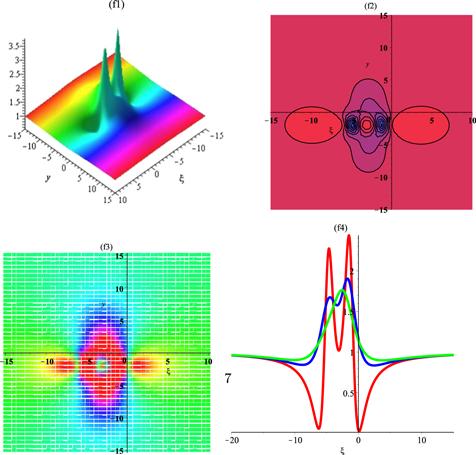
Figure 4. The second-order lump ( |
3.3. Set III: third-order solutions
We commence with three-wave functions based on the statement in step 2 in the previous section, and suppose that equation (1.5 ) has the rational function of third-order lump solutions. Taking n = 2 at (2.5 ), then (2.5 ) is expressed as $ \begin{eqnarray}\begin{array}{rcl}{\mathfrak{f}} & = & {{\mathfrak{f}}}_{3}(\xi ,y;\theta ,\delta )={\chi }_{3}(\xi ,y)+2\delta {{yp}}_{2}(\xi ,y)+2\delta \xi {s}_{2}(\xi ,y)\\ & & +({\theta }^{2}+{\delta }^{2}){\chi }_{1}(\xi ,y)={a}_{\mathrm{0,0}}+{\xi }^{12}\\ & & +2\,\theta \,\xi \left({\xi }^{6}{c}_{\mathrm{6,0}}+{\xi }^{4}{y}^{2}{c}_{\mathrm{4,2}}+{\xi }^{2}{y}^{4}{c}_{\mathrm{2,4}}+{y}^{6}{c}_{\mathrm{0,6}}\right.\\ & & \left.+{\xi }^{4}{c}_{\mathrm{4,0}}+{\xi }^{2}{y}^{2}{c}_{\mathrm{2,2}}+{y}^{4}{c}_{\mathrm{0,4}}+{\xi }^{2}{c}_{\mathrm{2,0}}+{y}^{2}{c}_{\mathrm{0,2}}+{c}_{\mathrm{0,0}}\right)\\ & & +{a}_{\mathrm{0,6}}{y}^{6}+{a}_{\mathrm{4,0}}{\xi }^{4}+{a}_{\mathrm{0,4}}{y}^{4}+{a}_{\mathrm{2,0}}{\xi }^{2}+{a}_{\mathrm{0,2}}{y}^{2}+{a}_{\mathrm{8,2}}{y}^{2}{\xi }^{8}\\ & & +{a}_{\mathrm{6,4}}{y}^{4}{\xi }^{6}+{a}_{\mathrm{8,4}}{y}^{4}{\xi }^{8}+{a}_{\mathrm{10,2}}{y}^{2}{\xi }^{10}+{a}_{\mathrm{4,8}}{y}^{8}{\xi }^{4}+{a}_{\mathrm{6,2}}{y}^{2}{\xi }^{6}\\ & & +{a}_{\mathrm{6,6}}{y}^{6}{\xi }^{6}+{a}_{\mathrm{4,4}}{y}^{4}{\xi }^{4}+{a}_{\mathrm{4,6}}{y}^{6}{\xi }^{4}+{a}_{\mathrm{2,8}}{y}^{8}{\xi }^{2}+{a}_{\mathrm{2,6}}{y}^{6}{\xi }^{2}\\ & & +{a}_{\mathrm{2,10}}{y}^{10}{\xi }^{2}+2\,\delta \,y({\xi }^{6}{b}_{\mathrm{6,0}}+{\xi }^{4}{y}^{2}{b}_{\mathrm{4,2}}+{\xi }^{2}{y}^{4}{b}_{\mathrm{2,4}}\\ & & +{y}^{6}{b}_{\mathrm{0,6}}+{\xi }^{4}{b}_{\mathrm{4,0}}+{\xi }^{2}{y}^{2}{b}_{\mathrm{2,2}}+{y}^{4}{b}_{\mathrm{0,4}}+{\xi }^{2}{b}_{\mathrm{2,0}}+{y}^{2}{b}_{\mathrm{0,2}}+{b}_{\mathrm{0,0}})\\ & & +{a}_{\mathrm{0,8}}{y}^{8}+{a}_{\mathrm{0,10}}{y}^{10}+{a}_{\mathrm{0,12}}{y}^{12}+\left({\delta }^{2}+{\theta }^{2}\right){\chi }_{1}(\xi ,y),\end{array}\end{eqnarray}$ where ${\chi }_{1}{(\xi ,y)=(\xi -\theta )}^{2}-\tfrac{c-{\gamma }_{1}}{{\gamma }_{3}}{(y-\delta )}^{2}+\tfrac{3\alpha }{c-{\gamma }_{1}}$ . Without loss of generality, we can choose a12,0 = 1. Plugging (3.13 ) into (3.1 ) and setting all the coefficients of the different powers of ${y}^{m}{\xi }^{m}$ to zero, we gain a system of nonlinear algebraic equations, and by solving the related system we arrive at the following parameters: $ \begin{eqnarray}\begin{array}{rcl}\alpha & = & -\displaystyle \frac{{a}_{\mathrm{10,0}}{a}_{\mathrm{10,2}}{\gamma }_{3}}{588},\ c=-\displaystyle \frac{1}{6}{a}_{\mathrm{10,2}}{\gamma }_{3}+{\gamma }_{1},\\ {a}_{\mathrm{0,0}} & = & \displaystyle \frac{\left(9\,150\,625{a}_{10,0}^{5}{a}_{10,2}^{3}+1129430400\,{\theta }^{2}{a}_{\mathrm{10,2}}{c}_{4,2}^{2}+21956126976{\delta }^{2}{b}_{4,2}^{2}\right){a}_{\mathrm{10,0}}}{83013134400{a}_{10,2}^{3}\left({\delta }^{2}+{\theta }^{2}+1\right)},\end{array}\end{eqnarray}$
$ \begin{eqnarray*}\begin{array}{rclcl}{a}_{\mathrm{0,2}} & = & \displaystyle \frac{32896875\,{a}_{10,0}^{5}{a}_{10,2}^{3}+1317668800\,{\theta }^{2}{a}_{\mathrm{10,2}}{c}_{4,2}^{2}+25615481472\,{\delta }^{2}{b}_{4,2}^{2}}{17788528800\,{a}_{10,2}^{2}\left({\delta }^{2}+{\theta }^{2}+1\right)},\,{a}_{\mathrm{0,4}} & = & \displaystyle \frac{334525\,{a}_{10,0}^{4}{a}_{10,2}^{2}}{203297472},\end{array}\end{eqnarray*}$
$ \begin{eqnarray*}\begin{array}{rcl}{a}_{\mathrm{0,6}} & = & \displaystyle \frac{28535\,{a}_{10,0}^{3}{a}_{10,2}^{3}}{21781872},\ \ {a}_{\mathrm{0,8}}=\displaystyle \frac{1445\,{a}_{10,0}^{2}{a}_{10,2}^{4}}{4148928},\\ {a}_{\mathrm{0,10}} & = & \displaystyle \frac{29\,{a}_{10,2}^{5}{a}_{\mathrm{10,0}}}{381024},\ \ {a}_{\mathrm{0,12}}=\displaystyle \frac{{a}_{10,2}^{6}}{46656},\end{array}\end{eqnarray*}$
$ \begin{eqnarray*}\begin{array}{rclcl}{a}_{\mathrm{2,0}} & = & \displaystyle \frac{2495625\,{a}_{10,0}^{5}{a}_{10,2}^{3}+188238400{\theta }^{2}{a}_{\mathrm{10,2}}{c}_{4,2}^{2}+3659354496\,{\delta }^{2}{b}_{4,2}^{2}}{423536400\,{a}_{10,2}^{3}\left({\delta }^{2}+{\theta }^{2}+1\right)},{a}_{\mathrm{2,2}} & = & \displaystyle \frac{275\,{a}_{10,0}^{4}{a}_{\mathrm{10,2}}}{268912},\end{array}\end{eqnarray*}$
$ \begin{eqnarray*}\begin{array}{rcl}{a}_{\mathrm{2,4}} & = & -\displaystyle \frac{25\,{a}_{10,0}^{3}{a}_{10,2}^{2}}{57624},\ \ {a}_{\mathrm{2,6}}=\displaystyle \frac{1265\,{a}_{10,0}^{2}{a}_{10,2}^{3}}{74088},\\ {a}_{\mathrm{2,8}} & = & \displaystyle \frac{95\,{a}_{\mathrm{10,0}}{a}_{10,2}^{4}}{21168},\ {a}_{\mathrm{2,10}}=\displaystyle \frac{{a}_{10,2}^{5}}{1296},\ {a}_{\mathrm{4,0}}=-\displaystyle \frac{15125\,{a}_{10,0}^{4}}{806736},\end{array}\end{eqnarray*}$
$ \begin{eqnarray*}\begin{array}{rcl}{a}_{\mathrm{4,2}} & = & \displaystyle \frac{375\,{a}_{\mathrm{10,2}}{a}_{10,0}^{3}}{9604},\ {a}_{\mathrm{4,4}}=\displaystyle \frac{2675\,{a}_{10,0}^{2}{a}_{10,2}^{2}}{24696},\\ {a}_{\mathrm{4,6}} & = & \displaystyle \frac{365\,{a}_{\mathrm{10,0}}{a}_{10,2}^{3}}{5292},\ {a}_{\mathrm{4,8}}=\displaystyle \frac{5\,{a}_{10,2}^{4}}{432},\ {a}_{\mathrm{6,0}}=\displaystyle \frac{55\,{a}_{10,0}^{3}}{2058},\end{array}\end{eqnarray*}$
$ \begin{eqnarray*}\begin{array}{rcl}{a}_{\mathrm{6,2}} & = & \displaystyle \frac{95\,{a}_{\mathrm{10,2}}{a}_{10,0}^{2}}{294},\ {a}_{\mathrm{6,4}}=\displaystyle \frac{55\,{a}_{\mathrm{10,0}}{a}_{10,2}^{2}}{126},\ {a}_{\mathrm{6,6}}=\displaystyle \frac{5\,{a}_{10,2}^{3}}{54},\\ {a}_{\mathrm{8,0}} & = & \displaystyle \frac{15\,{a}_{10,0}^{2}}{196},\ {a}_{\mathrm{8,2}}=\displaystyle \frac{115\,{a}_{\mathrm{10,0}}{a}_{\mathrm{10,2}}}{98},\ {a}_{\mathrm{8,4}}=\displaystyle \frac{5\,{a}_{10,2}^{2}}{12},\end{array}\end{eqnarray*}$
$ \begin{eqnarray*}{a}_{\mathrm{10,0}}={a}_{\mathrm{10,0}},\ {a}_{\mathrm{10,2}}={a}_{\mathrm{10,2}},\end{eqnarray*}$
$ \begin{eqnarray*}\begin{array}{rcl}{b}_{\mathrm{0,0}} & = & -\displaystyle \frac{11\,{a}_{10,0}^{3}{b}_{\mathrm{4,2}}}{1372\,{a}_{\mathrm{10,2}}},\ {b}_{\mathrm{0,2}}=\displaystyle \frac{{a}_{10,0}^{2}{b}_{\mathrm{4,2}}}{196},\ {b}_{\mathrm{0,4}}=\displaystyle \frac{{a}_{\mathrm{10,0}}{a}_{\mathrm{10,2}}{b}_{\mathrm{4,2}}}{420},\\ {b}_{\mathrm{0,6}} & = & -\displaystyle \frac{{a}_{10,2}^{2}{b}_{\mathrm{4,2}}}{180},\ {b}_{\mathrm{2,0}}=\displaystyle \frac{57\,{a}_{10,0}^{2}{b}_{\mathrm{4,2}}}{686\,{a}_{\mathrm{10,2}}},\end{array}\end{eqnarray*}$
$ \begin{eqnarray*}\begin{array}{rcl}{b}_{\mathrm{2,2}} & = & \displaystyle \frac{19\,{a}_{\mathrm{10,0}}{b}_{\mathrm{4,2}}}{49},\ {b}_{\mathrm{2,4}}=\displaystyle \frac{3}{10}{a}_{\mathrm{10,2}}{b}_{\mathrm{4,2}},\ {b}_{\mathrm{4,0}}=-\displaystyle \frac{9\,{a}_{\mathrm{10,0}}{b}_{\mathrm{4,2}}}{7\,{a}_{\mathrm{10,2}}},\\ {b}_{\mathrm{4,2}} & = & {b}_{\mathrm{4,2}},\ {b}_{\mathrm{6,0}}=-6\,\displaystyle \frac{{b}_{\mathrm{4,2}}}{{a}_{\mathrm{10,2}}},\ {c}_{\mathrm{0,0}}=-\displaystyle \frac{5\,{a}_{10,0}^{3}{c}_{\mathrm{4,2}}}{1764\,{a}_{\mathrm{10,2}}},\end{array}\end{eqnarray*}$
$ \begin{eqnarray*}\begin{array}{rcl}{c}_{\mathrm{0,2}} & = & -\displaystyle \frac{535\,{a}_{10,0}^{2}{c}_{\mathrm{4,2}}}{86436},\ {c}_{\mathrm{0,4}}=-\displaystyle \frac{5\,{a}_{\mathrm{10,0}}{a}_{\mathrm{10,2}}{c}_{\mathrm{4,2}}}{588},\\ {c}_{\mathrm{0,6}} & = & -\displaystyle \frac{5\,{a}_{10,2}^{2}{c}_{\mathrm{4,2}}}{324},\ {c}_{\mathrm{2,0}}=\displaystyle \frac{5\,{a}_{10,0}^{2}{c}_{\mathrm{4,2}}}{294\,{a}_{\mathrm{10,2}}},\\ {c}_{\mathrm{2,2}} & = & \displaystyle \frac{115\,{a}_{\mathrm{10,0}}{c}_{\mathrm{4,2}}}{441},\end{array}\end{eqnarray*}$
$ \begin{eqnarray*}\begin{array}{rcl}{c}_{\mathrm{2,4}} & = & \displaystyle \frac{5\,{a}_{\mathrm{10,2}}{c}_{\mathrm{4,2}}}{54},\ {c}_{\mathrm{4,0}}=-\displaystyle \frac{13\,{a}_{\mathrm{10,0}}{c}_{\mathrm{4,2}}}{147\,{a}_{\mathrm{10,2}}},\\ {c}_{\mathrm{4,2}} & = & {c}_{\mathrm{4,2}},\ {c}_{\mathrm{6,0}}=-\displaystyle \frac{2}{3}\displaystyle \frac{{c}_{\mathrm{4,2}}}{{a}_{\mathrm{10,2}}},\end{array}\end{eqnarray*}$
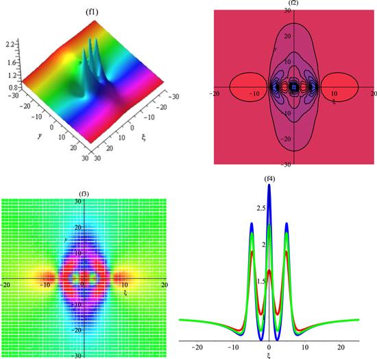
in which${b}_{\mathrm{4,2}}$ and ${c}_{\mathrm{4,2}}$ are arbitrary values. Thus, the third-order lump solutions of equation (1.5 ) can be obtained by $ \begin{eqnarray}{\rm{\Psi }}(\xi ,y)=2{\left(\mathrm{ln}{{\mathfrak{f}}}_{3}(\xi ,y;\theta ,\delta \right)}_{\xi \xi },\end{eqnarray}$ where ${{\mathfrak{f}}}_{3}(\xi ,y;\theta ,\delta )$ is given in equation (3.9 ). It is worth mentioning that this lump has the following features: $ \begin{eqnarray}\mathop{\mathrm{lim}}\limits_{\xi \longrightarrow \pm \infty }{\rm{\Psi }}(\xi ,y)={{\rm{\Psi }}}_{0},\ \ \ \mathop{\mathrm{lim}}\limits_{y\longrightarrow \pm \infty }{\rm{\Psi }}(\xi ,y)={{\rm{\Psi }}}_{0}.\end{eqnarray}$ By selecting suitable values of parameters, the graphical representation of periodic wave solution is presented in figures 5–7 including 3D plot, contour plot, density plot, and 2D plot where three spaces arise at spaces y = −1, y = 0, and y = 1. In figure 5 the rogue wave has one center $(\delta ,\theta )=(-2,-3)$ , while in figure 6 the lump has one center (δ, θ) = (2, 3), and in figure 7 the rogue wave has one center (δ, θ) = (0, 0).
in which
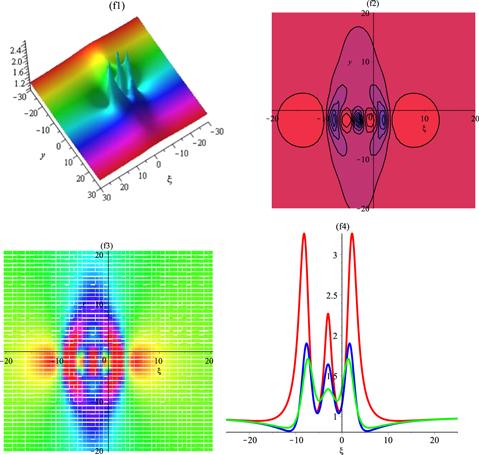
Figure 5. The three-order lump ( |
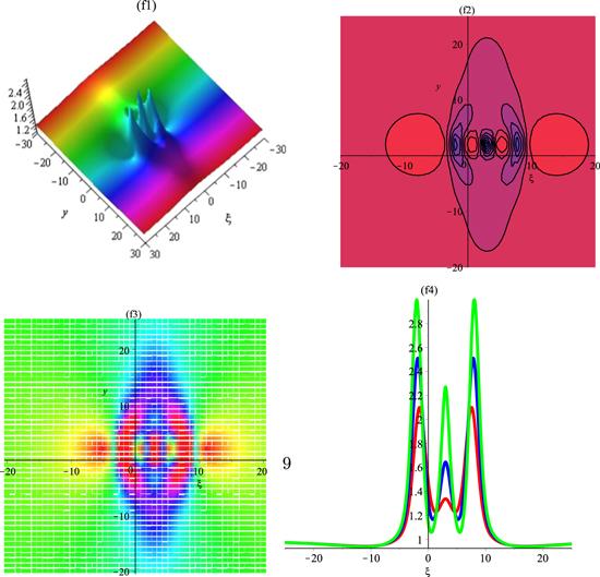
Figure 6. The three-order lump ( |
Figure 7. The three-order lump ( |
4. Application of SIVP for equation (1.5 )
By utilizing the wave transformation $\xi =k(x+y-{ct})$ in equation (1.5 ) one can arrive at a nonlinear ordinary differential equation as follows: $ \begin{eqnarray}\begin{array}{l}{k}^{2}(\alpha +\beta ){\rm{\Psi }}\unicode{x02057}+6k(\alpha +\beta ){\rm{\Psi }}^{\prime} {\rm{\Psi }}^{\prime\prime} \\ \quad +\,({\gamma }_{1}+{\gamma }_{2}+{\gamma }_{3}-c){\rm{\Psi }}^{\prime\prime} =0.\end{array}\end{eqnarray}$ Based on the semi-inverse variational principle [61–63], and by multiplying equation (4.1 ) with ${\rm{\Psi }}^{\prime} $ and integrating, we obtain the stationary integral $ \begin{eqnarray}\begin{array}{rcl}J & = & {\displaystyle \int }_{-\infty }^{\infty }\left(2k(\alpha +\beta ){\left({\rm{\Psi }}^{\prime} \right)}^{3}-\displaystyle \frac{1}{2}{k}^{2}(\alpha +\beta ){\left({\rm{\Psi }}^{\prime\prime} \right)}^{2}\right.\\ & & \left.+\displaystyle \frac{1}{2}({\gamma }_{1}+{\gamma }_{2}+{\gamma }_{3}-c){\left({\rm{\Psi }}^{\prime} \right)}^{2}+{k}^{2}(\alpha +\beta ){\rm{\Psi }}^{\prime} {\rm{\Psi }}\prime\prime\prime \right){\rm{d}}\xi .\end{array}\end{eqnarray}$
4.1. Case I
Using the solitary wave function as follows: $ \begin{eqnarray}u(\xi )=A\ {\rm{sech}} \left(B\xi \right).\end{eqnarray}$ Thus, the stationary integral changes to $ \begin{eqnarray}\begin{array}{rcl}J & = & \displaystyle \frac{1}{30}{A}^{2}B\left(-21\,{B}^{2}\alpha \,{k}^{2}-21\,{B}^{2}\beta \,{k}^{2}\right.\\ & & \left.-12\,{kAB}\alpha -12\,{kAB}\beta -5\,c+5\,{\gamma }_{1}+5\,{\gamma }_{2}+5\,{\gamma }_{3}\right),\end{array}\end{eqnarray}$ SIVP notes that the soliton amplitude and its inverse width are found according to the coupled system given below as $ \begin{eqnarray}\displaystyle \frac{\partial J}{\partial A}=0\end{eqnarray}$ and $ \begin{eqnarray}\displaystyle \frac{\partial J}{\partial B}=0,\end{eqnarray}$ and arrive at the following two nonlinear algebraic systems: $ \begin{eqnarray}\begin{array}{l}\displaystyle \frac{1}{15}{AB}\left(-21\,{B}^{2}\alpha \,{k}^{2}-21\,{B}^{2}\beta \,{k}^{2}-12\,{kAB}\alpha -12\,{kAB}\beta \right.\\ \quad \left.-\,5\,c+5\,{\gamma }_{1}+5\,{\gamma }_{2}+5\,{\gamma }_{3}\right)\\ \quad +\,\displaystyle \frac{1}{30}{A}^{2}B\left(-12\,B\alpha \,k-12\,B\beta \,k\right)=0,\end{array}\end{eqnarray}$ $ \begin{eqnarray}\begin{array}{l}\displaystyle \frac{1}{30}{A}^{2}\left(-21\,{B}^{2}\alpha \,{k}^{2}-21\,{B}^{2}\beta \,{k}^{2}-12\,{kAB}\alpha \right.\\ \quad \left.-\,12\,{kAB}\beta -5\,c+5\,{\gamma }_{1}+5\,{\gamma }_{2}+5{\gamma }_{3}\right)\\ \quad +\,\displaystyle \frac{1}{30}{A}^{2}B\left(-42\,B\alpha \,{k}^{2}-42B\beta \,{k}^{2}\right.\\ \quad -\,12\,A\alpha \,k-12\,A\beta \,k=0.\end{array}\end{eqnarray}$ By solving the above equations, one can recover a relation between these two parameters from (4.7 ) and (4.8 ) as $ \begin{eqnarray}\begin{array}{rcl}A & = & \pm \displaystyle \frac{1}{3}\displaystyle \frac{\left(c-{\gamma }_{1}-{\gamma }_{2}-{\gamma }_{3}\right)\sqrt{21}}{\sqrt{\left(\alpha +\beta \right)\left(c-{\gamma }_{1}-{\gamma }_{2}-{\gamma }_{3}\right)}},\\ B & = & \pm \displaystyle \frac{1}{21}\displaystyle \frac{\sqrt{21}\sqrt{\left(\alpha +\beta \right)\left(c-{\gamma }_{1}-{\gamma }_{2}-{\gamma }_{3}\right)}}{\left(\alpha +\beta \right)k}.\end{array}\end{eqnarray}$ The domain of definition of the above relations will be as $ \begin{eqnarray}\left(\alpha +\beta \right)\left(c-{\gamma }_{1}-{\gamma }_{2}-{\gamma }_{3}\right)\gt 0.\end{eqnarray}$ Lastly, the solitary wave solution acquired by means of SIVP will be as $ \begin{eqnarray}\begin{array}{l}{\rm{\Psi }}(x,y,t)=\pm \displaystyle \frac{1}{3}\displaystyle \frac{\left(c-{\gamma }_{1}-{\gamma }_{2}-{\gamma }_{3}\right)\sqrt{21}}{\sqrt{\left(\alpha +\beta \right)\left(c-{\gamma }_{1}-{\gamma }_{2}-{\gamma }_{3}\right)}}\ {\rm{sech}} \\ \times \,\left[\pm \displaystyle \frac{1}{21}\displaystyle \frac{\sqrt{21}\sqrt{\left(\alpha +\beta \right)\left(c-{\gamma }_{1}-{\gamma }_{2}-{\gamma }_{3}\right)}}{\left(\alpha +\beta \right)}(x+y-{ct})\right].\end{array}\end{eqnarray}$
4.2. Case II
We use the solitary wave function as follows: $ \begin{eqnarray}u(\xi )=A\ {{\rm{sech}} }^{2}(B\xi ).\end{eqnarray}$ Thus, the stationary integral changes to $ \begin{eqnarray}J=-\displaystyle \frac{\left(240\,{B}^{2}\alpha \,{k}^{2}+240\,{B}^{2}\beta \,{k}^{2}+70\,{kAB}\alpha +70\,{kAB}\beta +28\,c-28\,{\gamma }_{1}-28\,{\gamma }_{2}-28\,{\gamma }_{3}\right){A}^{2}B}{105}.\end{eqnarray}$ SIVP notes that the soliton amplitude and its inverse width are found according to the coupled system given below as $ \begin{eqnarray}\displaystyle \frac{\partial J}{\partial A}=-\displaystyle \frac{\left(70B\alpha k+70B\beta k\right){A}^{2}B}{105}-\displaystyle \frac{\left(480{B}^{2}\alpha {k}^{2}+480{B}^{2}\beta {k}^{2}+140{kAB}\alpha +140{kAB}\beta +56c-56{\gamma }_{1}-56\,{\gamma }_{2}-56{\gamma }_{3}\right){AB}}{105}=0\end{eqnarray}$ and $ \begin{eqnarray}\begin{array}{rcl}\displaystyle \frac{\partial J}{\partial B} & = & -\displaystyle \frac{\left(480\,B\alpha \,{k}^{2}+480\,B\beta \,{k}^{2}+70\,A\alpha \,k+70\,A\beta \,k\right){A}^{2}B}{105}\\ & & -\displaystyle \frac{\left(240\,{B}^{2}\alpha \,{k}^{2}+240\,{B}^{2}\beta \,{k}^{2}+70\,{kAB}\alpha +70\,{kAB}\beta +28\,c-28\,{\gamma }_{1}-28\,{\gamma }_{2}-28\,{\gamma }_{3}\right){A}^{2}}{105}=0.\end{array}\end{eqnarray}$ By solving the above equations, one can recover a relation between these two parameters from (4.14 ) and (4.15 ) as $ \begin{eqnarray}\begin{array}{rcl}A & = & \pm \displaystyle \frac{\left(16\,c-16\,{\gamma }_{1}-16\,{\gamma }_{2}-16\,{\gamma }_{3}\right)\sqrt{21}}{35\,\sqrt{\left(\alpha +\beta \right)\left(c-{\gamma }_{1}-{\gamma }_{2}-{\gamma }_{3}\right)}},\\ B & = & \pm \displaystyle \frac{1}{30}\displaystyle \frac{\sqrt{21}\sqrt{\left(\alpha +\beta \right)\left(c-{\gamma }_{1}-{\gamma }_{2}-{\gamma }_{3}\right)}}{\left(\alpha +\beta \right)k}.\end{array}\end{eqnarray}$ The domain of definition of the above relations will be as $ \begin{eqnarray}\left(\alpha +\beta \right)\left(c-{\gamma }_{1}-{\gamma }_{2}-{\gamma }_{3}\right)\gt 0.\end{eqnarray}$ Lastly, the bright wave solution acquired by means of SIVP will be as $ \begin{eqnarray}\begin{array}{l}{\rm{\Psi }}(x,y,t)=\pm \displaystyle \frac{\left(16\,c-16\,{\gamma }_{1}-16\,{\gamma }_{2}-16\,{\gamma }_{3}\right)\sqrt{21}}{35\,\sqrt{\left(\alpha +\beta \right)\left(c-{\gamma }_{1}-{\gamma }_{2}-{\gamma }_{3}\right)}}\ {{\rm{sech}} }^{2}\\ \times \,\left[\pm \displaystyle \frac{1}{30}\displaystyle \frac{\sqrt{21}\sqrt{\left(\alpha +\beta \right)\left(c-{\gamma }_{1}-{\gamma }_{2}-{\gamma }_{3}\right)}}{\left(\alpha +\beta \right)}(x+y-{ct})\right].\end{array}\end{eqnarray}$
4.3. Case III
Suppose the dark soliton wave solution takes the following form: $ \begin{eqnarray}u(\xi )=A\ {\tanh }^{2}(B\xi ).\end{eqnarray}$ Thus, the stationary integral changes to $ \begin{eqnarray}J=-\displaystyle \frac{2\,{A}^{2}B\left(-120\,{B}^{2}{{ck}}^{2}+35\,{kABc}-14\,S\right)}{105}.\end{eqnarray}$ SIVP notes that the soliton amplitude and its inverse width are found according to the coupled system given below as $ \begin{eqnarray}\displaystyle \frac{\partial J}{\partial A}=\displaystyle \frac{2\,{A}^{2}B\left(-120\,{B}^{2}\alpha \,{k}^{2}-120\,{B}^{2}\beta \,{k}^{2}+35\,{kAB}\alpha +35\,{kAB}\beta -14\,c+14\,{\gamma }_{1}+14\,{\gamma }_{2}+14\,{\gamma }_{3}\right)}{105}=0\end{eqnarray}$ and $ \begin{eqnarray}\begin{array}{rcl}\displaystyle \frac{\partial J}{\partial B} & = & \displaystyle \frac{2\,{A}^{2}\left(-120\,{B}^{2}\alpha \,{k}^{2}-120\,{B}^{2}\beta \,{k}^{2}+35\,{kAB}\alpha +35\,{kAB}\beta -14\,c+14\,{\gamma }_{1}+14\,{\gamma }_{2}+14\,{\gamma }_{3}\right)}{105}\\ & & +\displaystyle \frac{2\,{A}^{2}B\left(-240\,B\alpha \,{k}^{2}-240\,B\beta \,{k}^{2}+35\,A\alpha \,k+35A\beta \,k\right)}{105}=0.\end{array}\end{eqnarray}$ By solving the above equations, one can recover a relation between these two parameters from (4.21 ) and (4.22 ) as $ \begin{eqnarray}\begin{array}{rcl}A & = & \pm \displaystyle \frac{\left(16\,c-16\,{\gamma }_{1}-16\,{\gamma }_{2}-16\,{\gamma }_{3}\right)\sqrt{21}}{35\,\sqrt{\left(\alpha +\beta \right)\left(c-{\gamma }_{1}-{\gamma }_{2}-{\gamma }_{3}\right)}},\\ B & = & \pm \displaystyle \frac{1}{30}\displaystyle \frac{\sqrt{21}\sqrt{\left(\alpha +\beta \right)\left(c-{\gamma }_{1}-{\gamma }_{2}-{\gamma }_{3}\right)}}{\left(\alpha +\beta \right)k}.\end{array}\end{eqnarray}$ The domain of definition of the above relations will be as $ \begin{eqnarray}\left(\alpha +\beta \right)\left(c-{\gamma }_{1}-{\gamma }_{2}-{\gamma }_{3}\right)\gt 0.\end{eqnarray}$ Lastly, the dark wave solution acquired by the help of SIVP will be as $ \begin{eqnarray}\begin{array}{l}{\rm{\Psi }}(x,y,t)=\pm \displaystyle \frac{\left(16\,c-16\,{\gamma }_{1}-16\,{\gamma }_{2}-16\,{\gamma }_{3}\right)\sqrt{21}}{35\,\sqrt{\left(\alpha +\beta \right)\left(c-{\gamma }_{1}-{\gamma }_{2}-{\gamma }_{3}\right)}}\ {\tanh }^{2}\\ \times \,\left[\pm \displaystyle \frac{1}{30}\displaystyle \frac{\sqrt{21}\sqrt{\left(\alpha +\beta \right)\left(c-{\gamma }_{1}-{\gamma }_{2}-{\gamma }_{3}\right)}}{\left(\alpha +\beta \right)}(x+y-{ct})\right].\end{array}\end{eqnarray}$
5. Conclusion
In this article, we obtained multiple lump solutions and solitary, bright, and dark soliton solutions for the generalized Bogoyavlensky–Konopelchenko equation. The multiple lump solutions method contains first-order, second-order, and third-order wave solutions. At the critical point, the second-order derivative and Hessian matrix for only one point was investigated, and the lump solution for the first-order rouge wave solution obtained one maximum value. These results are beneficial for the study of gas, plasma, optics, acoustics, heat transfer, fluid dynamics, and classical mechanics. All calculations in this paper have been made using Maple.