


1. Introduction
| • | The nonlinear time-fractional coupled Whitham–Broer–Kaup (WBK) equations: $ \begin{eqnarray}\begin{array}{l}{T}_{t}^{\alpha }v+v{v}_{x}+{w}_{x}+\xi {v}_{xx}=0,\\ {T}_{t}^{\alpha }w+{(vw)}_{x}-\xi {w}_{xx}+\eta {v}_{xxx}=0.\end{array}\end{eqnarray}$ |
| • | The nonlinear time-fractional coupled Jaulent–Miodek (JM) equations: |
2. Notations and preliminaries
[21] Let f be n-differentiable at $t\gt s;$ the conformable fractional derivative starting from s of a function $f:\left(s,\infty \right]\to {\mathbb{R}}$ of order $\alpha \gt 0$ is defined by
[21] Let $\alpha \in (0,\,1]$ and assume $f,g$ be α-differentiable at a point $t\gt s.$ Then
| (1) $\displaystyle \frac{{{\rm{d}}}^{\alpha }}{{\rm{d}}{t}^{\alpha }}(kf\,+hg)\,=\,k{\rm{}}{f}^{\left(\alpha \right)}+h{\rm{}}{g}^{\left(\alpha \right)},k,\,h\in {\mathbb{R}}.$ | |
| (2) $\displaystyle \frac{{{\rm{d}}}^{\alpha }}{{\rm{d}}{t}^{\alpha }}\left(\lambda \right)=0,\lambda \in {\mathbb{R}}.$ | |
| (3) $\displaystyle \frac{{{\rm{d}}}^{\alpha }}{{\rm{d}}{t}^{\alpha }}\left(\lambda f\right)=\lambda \displaystyle \frac{{{\rm{d}}}^{\alpha }}{{\rm{d}}{t}^{\alpha }}\left(f\right).$ | |
| (4) $\displaystyle \frac{{{\rm{d}}}^{\alpha }}{{\rm{d}}{t}^{\alpha }}\left({\left(t-a\right)}^{p}\right)=\,p{\left(t-a\right)}^{p-\alpha },p\in {\mathbb{R}}.$ | |
| (5) If f is differentiable, then $\displaystyle \frac{{{\rm{d}}}^{\alpha }f}{{\rm{d}}{t}^{\alpha }}(t)={\left(t-a\right)}^{1-\alpha }\displaystyle \frac{{\rm{d}}f}{{\rm{d}}t}(t).$ |
[21] The conformable fractional integral starting from s of order $\alpha \in (n-1,n]$ of f is defined as
Let $\alpha \in (n-1,n]$ and assume f be n-times differentiable function. Then
| (1) $\displaystyle \frac{{{\rm{d}}}^{\alpha }}{{\rm{d}}{t}^{\alpha }}\left({I}_{s}^{\alpha }f\left(t\right)\right)=f\left(t\right).$ | |
| (2) ${I}_{s}^{\alpha }\left(\displaystyle \frac{{{\rm{d}}}^{\alpha }}{{\rm{d}}{t}^{\alpha }}f\left(t\right)\right)=f\left(t\right)-\displaystyle \sum _{k=0}^{n-1}\displaystyle \frac{{f}^{\left(k\right)}\left(s\right){\left(t-s\right)}^{k}}{k!}.$ |
[22] Let ${\partial }^{k}u/\partial {t}^{k}$ and ${\partial }^{k}u/\partial {x}^{k},$ $k\,=1,\,2,\,\ldots ,\,n-1$ be defined on $I\times \left[s,\infty \right),$ then the conformable time-fractional differential operator of order $\alpha \in \left(n-1,n\right]$ of a function $v\left(x,t\right):I\times [s,\infty )\to {\mathbb{R}}$ is defined by
[22] The conformable fractional integral starting from s of order $\alpha \in (n-1,n]$ of a function $v\left(x,t\right):I\,\times [s,\infty )\to {\mathbb{R}}$ is defined by
[43] For $0\leqslant n-1\lt \alpha \leqslant n,$ the power series of the form
For $0\leqslant n-1\lt \alpha \leqslant n,$ assume that $v\left(x,t\right):I\times [{t}_{0},{t}_{0}+{R}^{1/\alpha })\to {\mathbb{R}}$ can be expressed as the MFPS about $t={t}_{0}$ in the form
Let $v\left(x,t\right)$ be a function of two variables that can be expressed as the MFPS of equation (
Let $\alpha \in (n-1,n],$ ${T}_{t}^{k\alpha }v\left(x,t\right)$ exist at a neighborhood of a point ${t}_{0}$ for $k=0,1,2,\ldots ,n+1,$ and $v\left(x,t\right)$ can be expressed by the MFPS (
From the assumption that $\left|{T}_{t}^{(n+1)\alpha }v\left(x,t\right)\right|\leqslant M(x),$ it follows
3. Detailed steps of CRPS method
Suppose that the solutions of the nonlinear FPDEs (
According to the initial conditions (
Define the nth-truncated residual functions as follows:
Substitute the nth-truncated MFPS solution (
Set $n=1$ in equation (
For $n=2,3,\ldots ,N,$ applying the operator ${T}_{t}^{\alpha },$ ($n-1$)-times, on both sides of equation (
Collect the obtained coefficients ${f}_{i,n}\left(x\right)$ and ${v}_{i,n}\left(x,t\right)$ for each $n=0,1,2,\ldots ,N$ in term of expanded MFPS and try to find a general pattern with the term infinite series so that the exact solution ${v}_{i}\left(x,t\right)$ of FPDEs (
Let ${v}_{i}\left(x,t\right),i=1,2,$ be the exact solutions of FPDEs (
For all $x\in I$ and $t\in \left[{t}_{0},{t}_{0}+{R}^{1/\alpha }\right],$ let ${f}_{i,0}\left(x\right)={v}_{i}\left(x,0\right),$ then from $\parallel {v}_{i,n+1}\left(x,t\right)\parallel \leqslant {\rho }_{i}\parallel {v}_{i,n}\left(x,t\right)\parallel ,$ we have $\parallel {v}_{i,1}\left(x,t\right)\parallel \leqslant {\rho }_{i}\parallel {v}_{i,0}\left(x,t\right)\parallel ={\rho }_{i}\parallel {f}_{i,0}\left(x\right)\parallel .$ Similarly, $\parallel {v}_{i,2}\left(x,t\right)\parallel $ $\leqslant {\rho }_{i}\parallel {v}_{i,1}\left(x,t\right)\parallel \leqslant {{\rho }_{i}}^{2}\parallel {f}_{i,0}\left(x\right)\parallel .$ Thus, $\parallel {v}_{i,k}\left(x,t\right)\parallel \,\leqslant {\rho }_{i}^{k}\parallel {f}_{i,0}\left(x\right)\parallel $ and $\displaystyle {\sum }_{k=n+1}^{\infty }\parallel {v}_{i,k}\left(x,t\right)\parallel \leqslant \displaystyle {\sum }_{k=n+1}^{\infty }{\rho }_{i}^{k}\parallel {f}_{i,0}\left(x\right)\parallel $ = ${f}_{i,0}\left(x\right)\displaystyle {\sum }_{k=n+1}^{\infty }{\rho }_{i}^{k}.$ Consequently, we have
4. Numerical simulation of physical models
Consider the nonlinear fractional coupled WBK system [48]:
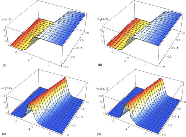
Figure 1. Comparison of exact and 6th-CRPS approximate graphs of the coupled WBK system ( |
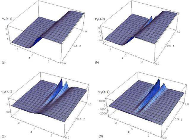
Figure 2. Surface waves plots of CRPS solution, ${v}_{6}\left(x,t\right),$ of equation ( |
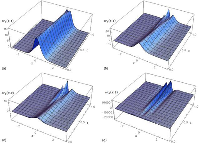
Figure 3. Surface waves plots of CRPS solution, ${w}_{6}\left(x,t\right),$ of equation ( |
Table 1. Errors results for the 7th-CRPS of coupled system ( |
| $v\left(x,t\right)$ solution | $w\left(x,t\right)$ solution | |||
|---|---|---|---|---|
| ${t}_{i}$ | Absolute error | Relative error | Absolute error | Relative error |
| $0.2$ | $9.50351\times {10}^{-13}$ | $1.11807\times {10}^{-13}$ | $3.7905\times {10}^{-12}$ | $1.13844\times {10}^{-9}$ |
| $0.4$ | $2.54341\times {10}^{-10}$ | $2.99229\times {10}^{-11}$ | $1.01636\times {10}^{-9}$ | $2.04618\times {10}^{-8}$ |
| $0.6$ | $6.84333\times {10}^{-9}$ | $8.05115\times {10}^{-10}$ | $2.73447\times {10}^{-8}$ | $3.69024\times {10}^{-7}$ |
| $0.8$ | $7.18967\times {10}^{-8}$ | $8.45871\times {10}^{-9}$ | $2.87265\times {10}^{-7}$ | $2.59868\times {10}^{-6}$ |
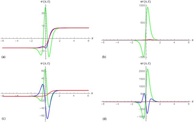
Figure 4. Comparison of exact solutions with CRPS method and LADM [48] in 2D for system ( |
Consider the nonlinear fractional coupled JM system [28]:
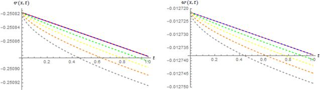
Figure 5. Graphs of exact and CRPS solution behavior of coupled MB system ( |
Table 2. Comparison of absolute errors, ${v}_{2}(x,t),$ of system ( |
| ${t}_{i}$ | ${x}_{i}$ | CRPS method | OHAM [49] | ADM [50] |
|---|---|---|---|---|
| $0.1$ | $0.1$ | $2.41474\times {10}^{-14}$ | $6.35267\times {10}^{-5}$ | $8.16297\times {10}^{-7}$ |
| $0.3$ | $2.23710\times {10}^{-14}$ | $1.90854\times {10}^{-4}$ | $7.64245\times {10}^{-7}$ | |
| $0.5$ | $2.07057\times {10}^{-14}$ | $3.18548\times {10}^{-4}$ | $7.16083\times {10}^{-7}$ | |
| $0.3$ | $0.1$ | $6.53311\times {10}^{-13}$ | $6.03098\times {10}^{-5}$ | $7.33445\times {10}^{-6}$ |
| $0.3$ | $6.04128\times {10}^{-13}$ | $1.81187\times {10}^{-4}$ | $6.86758\times {10}^{-6}$ | |
| $0.5$ | $5.59441\times {10}^{-13}$ | $3.02408\times {10}^{-4}$ | $6.43557\times {10}^{-6}$ | |
| $0.5$ | $0.1$ | $3.02491\times {10}^{-12}$ | $5.72865\times {10}^{-5}$ | $2.03415\times {10}^{-5}$ |
| $0.3$ | $2.79698\times {10}^{-12}$ | $1.72102\times {10}^{-4}$ | $1.90489\times {10}^{-5}$ | |
| $0.5$ | $2.59009\times {10}^{-12}$ | $2.87240\times {10}^{-4}$ | $1.78528\times {10}^{-5}$ |
Table 3. Comparison of absolute errors, ${w}_{2}(x,t),$ of system ( |
| ${t}_{i}$ | ${x}_{i}$ | CRPS method | OHAM [49] | ADM [50] |
|---|---|---|---|---|
| $0.1$ | $0.1$ | $9.57047\times {10}^{-15}$ | $1.65942\times {10}^{-5}$ | $5.88676\times {10}^{-5}$ |
| $0.3$ | $8.67188\times {10}^{-15}$ | $4.98691\times {10}^{-5}$ | $5.56914\times {10}^{-5}$ | |
| $0.5$ | $7.88952\times {10}^{-15}$ | $8.26491\times {10}^{-4}$ | $5.27169\times {10}^{-5}$ | |
| $0.3$ | $0.1$ | $2.58368\times {10}^{-13}$ | $1.55880\times {10}^{-5}$ | $1.78041\times {10}^{-4}$ |
| $0.3$ | $2.34352\times {10}^{-13}$ | $4.68439\times {10}^{-5}$ | $1.68429\times {10}^{-4}$ | |
| $0.5$ | $2.12989\times {10}^{-13}$ | $7.63646\times {10}^{-4}$ | $1.59428\times {10}^{-4}$ | |
| $0.5$ | $0.1$ | $1.19627\times {10}^{-12}$ | $1.46569\times {10}^{-5}$ | $2.99162\times {10}^{-4}$ |
| $0.3$ | $1.08511\times {10}^{-12}$ | $4.40448\times {10}^{-5}$ | $2.83001\times {10}^{-4}$ | |
| $0.5$ | $9.86156\times {10}^{-12}$ | $7.06678\times {10}^{-4}$ | $2.67868\times {10}^{-4}$ |
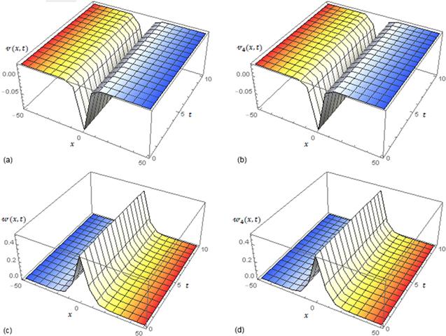
Figure 6. Surface graphs of exact and 4th-CRPS solutions for example 2 at $\alpha =1,$ $c=0.5,$ $0\leqslant t\leqslant 10,$ and $-50\leqslant x\leqslant 50:$ (a) exact solution $v(x,t);$ (b) CRPS solution ${v}_{4}\left(x,t\right);$ (c) exact solution $w(x,t);$ and (d) CRPS solution ${w}_{4}\left(x,t\right).$ |
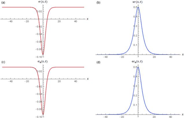
Figure 7. Nature of exact and 4th-CRPS solutions in 2D for example 2 at $=1,$ $c=0.5,$ $t=1,$ and $-50\leqslant x\leqslant 50:$ (a) exact solutions $v(x,t);$ (b) exact solutions $w(x,t);$ (c) CRPS solutions ${v}_{4}(x,t);$ and (d) CRPS solutions ${w}_{4}(x,t).$ |
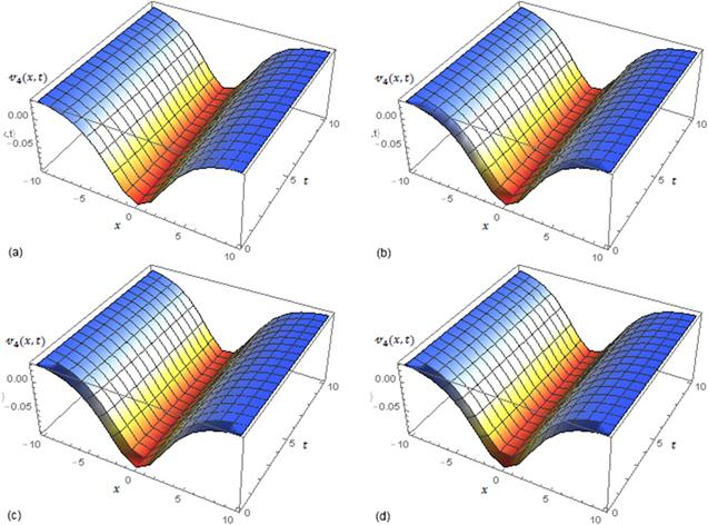
Figure 8. Surface graphs of 4th-CRPS solutions, ${v}_{4}\left(x,t\right),$ of Example 2 at different fractional-order levels for $c=0.25,$ $0\leqslant t\leqslant 10,$ and $-10\leqslant x\leqslant 10:$ (a) $\alpha =1;$ (b) $\alpha =0.75;$ (c) $\alpha =0.5;$ and (d) $\alpha =0.25.$ |
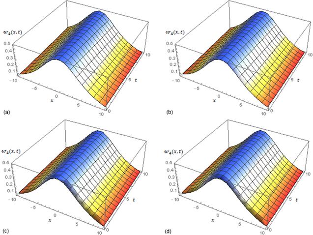
Figure 9. Surface graphs of 4th-CRPS solutions, ${w}_{4}\left(x,t\right),$ of Example 2 at different fractional-order levels for $c=0.25,$ $0\leqslant t\leqslant 10,$ and $-10\leqslant x\leqslant 10:$ (a) $\alpha =1;$ (b) $\alpha =0.75;$ (c) $\alpha =0.5;$ and (d) $\alpha =0.25.$ |