


1. Introduction
In some branches of science and engineering such as fluid mechanics, quantum mechanics, particle physics, mass transfer, plasma physics, nano liquids and biological mathematics [1–5], nonlinear partial differential equations (NPDES) are used to describe many nonlinear phenomena and wave propagation characteristics. As the lump solutions of the NPDES are the special, powerful destructive ocean wave in the real world, it is important to search for the lump solutions of the NPDES, especially the constant-coefficient NPDES that have attracted the attention of many scholars [6–10].
Recently, a generalized (3 + 1)-dimensional nonlinear-wave equation has been presented as [11]
$ \begin{eqnarray}{\left[4{u}_{t}+4{{uu}}_{x}+{u}_{{xxx}}-4{u}_{x}\right]}_{x}+3({u}_{{yy}}+{u}_{{zz}})=0,\end{eqnarray}$
which describes a liquid with gas bubbles in the three-dimensional case.However, the variable-coefficient NPDES provide us with more real phenomena in the inhomogeneities of media and non-uniformities of boundaries than corresponding constant-coefficient counterparts in some physical cases [12–15]. In this paper, a generalized (3 + 1)-dimensional variable-coefficient nonlinear-wave equation is investigated [16, 17]2 ) have not been obtained yet, which will make the main work of our paper.
$ \begin{eqnarray}\begin{array}{l}\alpha (t){u}_{x}^{2}+\alpha (t){{uu}}_{{xx}}+\beta (t){u}_{{xxxx}}+\gamma (t){u}_{{xx}}\\ \quad +\,\delta (t){u}_{{yy}}+\varrho (t){u}_{{zz}}+{u}_{{xt}}=0,\end{array}\end{eqnarray}$
where u = u(x, y, z, t) is the wave-amplitude function. The bilinear form, Bäcklund transformation, Lax pair, infinitely-many conservation laws, multi-soliton solutions, traveling-wave solutions and one-periodic wave solutions are presented by virtue of the binary Bell polynomials, the Hirota method, the polynomial expansion method and the Hirota-Riemann method [18]. However, lump and interaction solutions between the lump and solitary wave of equation (This paper will be organized as follows: section 2 obtains the lump solutions of equation (2 ) with the aid of the Hirota's bilinear form [19–24] and demonstrates their physical structures by some 3D plots; section 3 presents the interaction solutions between lump and one solitary wave; section 4 derives the interaction solutions between lump and two solitary waves; and section 5 gives the conclusion.
2. Lump solutions of equation (2 )
Setting $u=12\,{[\mathrm{ln}\xi (x,y,z,t)]}_{{xx}}$ and α(t) = β(t), and using the multi-dimensional Bell polynomials, the bilinear form of equation (2 ) can be introduced as (see [18])
$ \begin{eqnarray}\left[{{\rm{D}}}_{x}{{\rm{D}}}_{t}+\beta (t){{\rm{D}}}_{x}^{4}+\gamma (t){{\rm{D}}}_{x}^{2}+\delta (t){{\rm{D}}}_{y}^{2}+\varrho (t){{\rm{D}}}_{z}^{2}\right]\xi \cdot \xi =0.\end{eqnarray}$
This is equivalent to2 ), we suppose5 ) into equation (4 ) through Mathematica software, we get5 ) and (6 ) into the transformation $u=12\,{[\mathrm{ln}\xi (x,y,z,t)]}_{{xx}}$, we have the following lump solution of equation (2 )
$ \begin{eqnarray}\begin{array}{l}\xi [\beta (t){\xi }_{{xxxx}}+\gamma (t){\xi }_{{xx}}+\delta (t){\xi }_{{yy}}+\varrho (t){\xi }_{{zz}}+{\xi }_{{xt}}]\\ \qquad +\ 3\beta (t){\xi }_{{xx}}^{2}-4\beta (t){\xi }_{x}{\xi }_{{xxx}}-\gamma (t){\xi }_{x}^{2}\\ \qquad -\ \delta (t){\xi }_{y}^{2}-\varrho (t){\xi }_{z}^{2}-{\xi }_{t}{\xi }_{x}=0.\end{array}\end{eqnarray}$
In order to seek the lump solutions of equation ( $ \begin{eqnarray}\begin{array}{rcl}\zeta & = & x{\alpha }_{1}+y{\alpha }_{2}+z{\alpha }_{3}+{\alpha }_{4}(t),\\ \varsigma & = & x{\alpha }_{5}+y{\alpha }_{6}+z{\alpha }_{7}+{\alpha }_{8}(t),\\ \xi & = & {\zeta }^{2}+{\varsigma }^{2}+{\alpha }_{9}(t),\end{array}\end{eqnarray}$
where α1, α2, α3, α5, α6 and α7 are unknown constants. α4(t), α8(t) and α9(t) are undefined real functions. Substituting equation ( $ \begin{eqnarray}\begin{array}{rcl}(I):{\alpha }_{8}(t) & = & {\eta }_{1}\,-\,\int \displaystyle \frac{\left({\alpha }_{1}^{2}+{\alpha }_{5}^{2}\right)\left[{\alpha }_{1}^{2}\right.\gamma (t)+{\alpha }_{2}^{2}\delta (t)+{\alpha }_{3}^{2}\varrho (t)]+{\alpha }_{1}^{3}{\alpha }_{4}^{{\prime} }(t)}{{\alpha }_{1}^{2}{\alpha }_{5}}\,{\rm{d}}t,\\ {\alpha }_{9}(t) & = & {\eta }_{2}+\int \left[2[\right.{\alpha }_{1}\left({\alpha }_{1}\gamma (t)+{\alpha }_{4}^{{\prime} }(t\right)\,+\,{\alpha }_{2}^{2}\delta (t)+{\alpha }_{3}^{2}\varrho (t)][{\alpha }_{1}[{\eta }_{3}\\ & - & \,\left.\int \displaystyle \frac{\left({\alpha }_{1}^{2}+{\alpha }_{5}^{2}\right)[{\alpha }_{1}^{2}\gamma (t)+{\alpha }_{2}^{2}\delta (t)+{\alpha }_{3}^{2}\varrho (t)]+{\alpha }_{1}^{3}{\alpha }_{4}^{{\prime} }(t)}{{\alpha }_{1}^{2}{\alpha }_{5}}\,{\rm{d}}t\right]-{\alpha }_{5}\ast \ {\alpha }_{4}(t)]]/({\alpha }_{1}{\alpha }_{5})\,{\rm{d}}t,\alpha (t)=\beta (t)=0,\\ {\alpha }_{6} & = & \displaystyle \frac{{\alpha }_{2}{\alpha }_{5}}{{\alpha }_{1}},{\alpha }_{7}=\displaystyle \frac{{\alpha }_{3}{\alpha }_{5}}{{\alpha }_{1}},\end{array}\end{eqnarray}$
with ${\alpha }_{1}\ne 0$, ${\alpha }_{5}\ne 0$. Substituting equations ( $ \begin{eqnarray}\begin{array}{rcl}{u}^{(I)} & = & \left[12\left[2\left({\alpha }_{1}^{2}+{\alpha }_{5}^{2}\right)\left[{\eta }_{2}+\int \left[2\left[{\alpha }_{1}\left[{\alpha }_{1}\gamma (t)+{\alpha }_{4}^{{\prime} }(t)\right]\right.\right.\right.\right.\right.\left.+\,{\alpha }_{2}^{2}\delta (t)+{\alpha }_{3}^{2}\varrho (t)\right]\left[{\alpha }_{1}\left[{\eta }_{1}\right.\right.\\ & - & \,\left.\int \displaystyle \frac{\left({\alpha }_{1}^{2}+{\alpha }_{5}^{2}\right)\left[{\alpha }_{1}^{2}\gamma (t)+{\alpha }_{2}^{2}\delta (t)+{\alpha }_{3}^{2}\varrho (t)\right]+{\alpha }_{1}^{3}{\alpha }_{4}^{{\prime} }(t)}{{\alpha }_{1}^{2}{\alpha }_{5}}\,{\rm{d}}t\right]\left.\left.-\,{\alpha }_{5}{\alpha }_{4}(t)\right]\right]/({\alpha }_{1}{\alpha }_{5})\,{\rm{d}}t\\ & + & \,\left[{\eta }_{1}-\int \displaystyle \frac{\left({\alpha }_{1}^{2}+{\alpha }_{5}^{2}\right)\left[{\alpha }_{1}^{2}\gamma (t)+{\alpha }_{2}^{2}\delta (t)+{\alpha }_{3}^{2}\varrho (t)\right]+{\alpha }_{1}^{3}{\alpha }_{4}^{{\prime} }(t)}{{\alpha }_{1}^{2}{\alpha }_{5}}\,{\rm{d}}t\right.\\ & + & \left.\left.\,\displaystyle \frac{{\alpha }_{5}\left({\alpha }_{1}x+{\alpha }_{2}y+{\alpha }_{3}z\right)}{{\alpha }_{1}}\right]{}^{2}+\left[{\alpha }_{4}(t)+{\alpha }_{1}x+{\alpha }_{2}y+{\alpha }_{3}z\right]{}^{2}\right]-4\left[{\alpha }_{5}\left[{\eta }_{1}\right.\right.\\ & - & \left.\,\int \displaystyle \frac{\left({\alpha }_{1}^{2}+{\alpha }_{5}^{2}\right)\left[{\alpha }_{1}^{2}\gamma (t)+{\alpha }_{2}^{2}\delta (t)+{\alpha }_{3}^{2}\varrho (t)\right]+{\alpha }_{1}^{3}{\alpha }_{4}^{{\prime} }(t)}{{\alpha }_{1}^{2}{\alpha }_{5}}\,{\rm{d}}t+{\alpha }_{5}x\right]\left.\left.\left.+\,{\alpha }_{1}\left({\alpha }_{4}(t)+{\alpha }_{2}y+{\alpha }_{3}z\right)+{\alpha }_{1}^{2}x+\displaystyle \frac{{\alpha }_{5}^{2}\left({\alpha }_{2}y+{\alpha }_{3}z\right)}{{\alpha }_{1}}\right]{}^{2}\right]\right]/\left[\left[{\eta }_{2}\right.\right.\\ & + & \,\int \left[2\left[{\alpha }_{1}\left({\alpha }_{1}\gamma (t)+{\alpha }_{4}^{{\prime} }(t\right)+{\alpha }_{2}^{2}\delta (t)+{\alpha }_{3}^{2}\varrho (t)\right]\left[{\alpha }_{1}\left[{\eta }_{1}\right.\right.\right.\left.-\,\int \displaystyle \frac{\left({\alpha }_{1}^{2}+{\alpha }_{5}^{2}\right)\left[{\alpha }_{1}^{2}\gamma (t)+{\alpha }_{2}^{2}\delta (t)+{\alpha }_{3}^{2}\varrho (t)\right]+{\alpha }_{1}^{3}{\alpha }_{4}^{{\prime} }(t)}{{\alpha }_{1}^{2}{\alpha }_{5}}\,{\rm{d}}t\right]\\ & - & \left.\left.\,{\alpha }_{5}{\alpha }_{4}(t)\right]\right]/({\alpha }_{1}{\alpha }_{5})\,{\rm{d}}t\,+\,\left[{\eta }_{1}-\int \displaystyle \frac{\left({\alpha }_{1}^{2}+{\alpha }_{5}^{2}\right)\left[{\alpha }_{1}^{2}\gamma (t)+{\alpha }_{2}^{2}\delta (t)+{\alpha }_{3}^{2}\varrho (t)\right]+{\alpha }_{1}^{3}{\alpha }_{4}^{{\prime} }(t)}{{\alpha }_{1}^{2}{\alpha }_{5}}\,{\rm{d}}t\right.\\ & + & \left.\left.\left.\,\displaystyle \frac{{\alpha }_{5}\left({\alpha }_{1}x+{\alpha }_{2}y+{\alpha }_{3}z\right)}{{\alpha }_{1}}\right]{}^{2}+\left({\alpha }_{4}(t)+{\alpha }_{1}x+{\alpha }_{2}y+{\alpha }_{3}z\right){}^{2}\right]{}^{2}\right],\end{array}\end{eqnarray}$
where α4(t) is arbitrary function, η1 and η2 are integral constants.The physical structures for $({u}^{(I)})$ are described in figure 1 by the 3D plots. Figure 1 shows the propagation of solution $({u}^{(I)})$ when γ(t), δ(t), ϱ(t) and α4(t) select different functions. When $\gamma (t)=\delta (t)=\varrho (t)=\cos t$ and ${\alpha }_{4}(t)=\sin t$, a periodic-shape rational solution is listed in figure 1(a). When γ (t) = δ(t) = ϱ(t) = t and ${\alpha }_{4}(t)\,=\sin \ t$, a parabolic-shape rational solution is presented in figure 1(b). When $\gamma (t)=\cosh t,\varrho (t)=\exp \,t$ and ${\alpha }_{4}(t)\,=\delta (t)=t$, a cubic-shape rational solution is shown in figure 1(c).5 ) and (8 ) into the transformation $u=12\,{[\mathrm{ln}\xi (x,y,z,t)]}_{{xx}}$, we have the following lump solution of equation (2 )
$ \begin{eqnarray}\begin{array}{rcl}({II}):{\alpha }_{8}(t) & = & {\eta }_{3}+\int {\alpha }_{5}\left[-\displaystyle \frac{3\left({\alpha }_{1}^{2}+{\alpha }_{5}^{2}\right)\beta (t)}{{\alpha }_{9}}\right.\\ & & \left.-\displaystyle \frac{{\alpha }_{3}^{2}\varrho (t)}{{\alpha }_{1}^{2}}-\gamma (t)\right]\,{\rm{d}}t,\\ {\alpha }_{9}(t) & = & {\alpha }_{9},{\alpha }_{6}=-\displaystyle \frac{{\alpha }_{1}{\alpha }_{2}}{{\alpha }_{5}},{\alpha }_{7}=\displaystyle \frac{{\alpha }_{3}{\alpha }_{5}}{{\alpha }_{1}},\\ \delta (t) & = & -\displaystyle \frac{3{\alpha }_{5}^{2}\left({\alpha }_{1}^{2}+{\alpha }_{5}^{2}\right)\beta (t)}{{\alpha }_{2}^{2}{\alpha }_{9}},\\ {\alpha }_{4}(t) & = & {\eta }_{4}-\int \left[\displaystyle \frac{{\alpha }_{1}[3\left({\alpha }_{1}^{2}+{\alpha }_{5}^{2}\right)\beta (t)+{\alpha }_{9}\gamma (t)]}{{\alpha }_{9}}\right.\\ & & \left.+\displaystyle \frac{{\alpha }_{3}^{2}\varrho (t)}{{\alpha }_{1}}\right]\,{\rm{d}}t,\end{array}\end{eqnarray}$
with ${\alpha }_{1}\ne 0$, ${\alpha }_{5}\ne 0$, ${\alpha }_{9}\ne 0$ and ${\alpha }_{2}{\alpha }_{9}\ne 0$. Substituting equations ( $ \begin{eqnarray}\begin{array}{rcl}\,{u}^{({II})} & = & \left[12\left[2\left({\alpha }_{1}^{2}+{\alpha }_{5}^{2}\right)\left[{\alpha }_{9}+\left[\int {\alpha }_{5}\left[-\displaystyle \frac{3\left({\alpha }_{1}^{2}+{\alpha }_{5}^{2}\right)\beta (t)}{{\alpha }_{9}}\right.\right.\right.\right.\right.\\ & & \left.-\displaystyle \frac{{\alpha }_{3}^{2}\varrho (t)}{{\alpha }_{1}^{2}}-\gamma (t)\right]\,{\rm{d}}t+\left.{\eta }_{3}+{\alpha }_{5}x-\displaystyle \frac{{\alpha }_{1}{\alpha }_{2}y}{{\alpha }_{5}}+\displaystyle \frac{{\alpha }_{3}{\alpha }_{5}z}{{\alpha }_{1}}\right]{}^{2}\\ & & +\left[\int \left[-\displaystyle \frac{{\alpha }_{1}[3\left({\alpha }_{1}^{2}+{\alpha }_{5}^{2}\right)\beta (t)+{\alpha }_{9}\gamma (t)]}{{\alpha }_{9}}\right.\right.\\ & & \left.-\displaystyle \frac{{\alpha }_{3}^{2}\varrho (t)}{{\alpha }_{1}}\right]\,{\rm{d}}t+{\eta }_{4}+{\alpha }_{1}x+{\alpha }_{2}y+{\alpha }_{3}z]{}^{2}]\\ & & -\left[4\left[{\alpha }_{1}^{2}\left[\int \left[-\displaystyle \frac{{\alpha }_{1}\left[3\left({\alpha }_{1}^{2}+{\alpha }_{5}^{2}\right)\beta (t)+{\alpha }_{9}\gamma (t)\right]}{{\alpha }_{9}}\right.\right.\right.\right.\\ & & \left.\left.-\displaystyle \frac{{\alpha }_{3}^{2}\varrho (t)}{{\alpha }_{1}}\right]\,{\rm{d}}t\right]+{\alpha }_{5}{\alpha }_{1}\left[{\eta }_{3}\right.\\ & & +\int {\alpha }_{5}\left[-\displaystyle \frac{3\left({\alpha }_{1}^{2}+{\alpha }_{5}^{2}\right)\beta (t)}{{\alpha }_{9}}-\displaystyle \frac{{\alpha }_{3}^{2}\varrho (t)}{{\alpha }_{1}^{2}}-\gamma (t)\right]\,{\rm{d}}t\\ & & \left.+{\alpha }_{5}x\right]+{\alpha }_{1}^{3}x\\ & & +{\alpha }_{1}^{2}\left({\eta }_{4}+{\alpha }_{3}z\right)+{\alpha }_{3}{\alpha }_{5}^{2}z]{}^{2}]/({\alpha }_{1}^{2})]]\\ & & \,/\left[\left[{\alpha }_{9}+\left[{\eta }_{3}+{\alpha }_{5}x-\displaystyle \frac{{\alpha }_{1}{\alpha }_{2}y}{{\alpha }_{5}}+\displaystyle \frac{{\alpha }_{3}{\alpha }_{5}z}{{\alpha }_{1}}\right.\right.\right.\\ & & \left.+\int {\alpha }_{5}\left[-\displaystyle \frac{3\left({\alpha }_{1}^{2}+{\alpha }_{5}^{2}\right)\beta (t)}{{\alpha }_{9}}-\displaystyle \frac{{\alpha }_{3}^{2}\varrho (t)}{{\alpha }_{1}^{2}}-\gamma (t)\right]\,{\rm{d}}t\right]{}^{2}\\ & & +[{\eta }_{4}+{\alpha }_{1}x+{\alpha }_{2}y\\ & & -\int \left[\displaystyle \frac{{\alpha }_{1}[3\left({\alpha }_{1}^{2}+{\alpha }_{5}^{2}\right)\beta (t)+{\alpha }_{9}\gamma (t)]}{{\alpha }_{9}}+\displaystyle \frac{{\alpha }_{3}^{2}\varrho (t)}{{\alpha }_{1}}\right]\,{\rm{d}}t\\ & & \left.\left.\left.+{\alpha }_{3}z\right]{}^{2}\right]{}^{2}\right],\end{array}\end{eqnarray}$
where η3 and η4 are integral constants.
Figure 1. Lump solution u(I) with α1 = 1, α2 = 2, α3 = −1, α5 = −3, x = −5, η1 = η2 = y = 0, when $\gamma (t)=\delta (t)=\varrho (t)\,=\cos t,{\alpha }_{4}(t)=\sin t$ in (a), $\gamma (t)=\delta (t)=\varrho (t)=t,{\alpha }_{4}(t)=\sin t$ in (b) and $\gamma (t)=\cosh t$, $\varrho (t)=\exp \,t$ and α4(t) = δ(t) = t in (c). |
Then, the physical structures for $({u}^{({II})})$ are shown in figures 2–5 with some 3D plots. When $\gamma (t)\,=-1,\varrho (t)=\beta (t)=1$, the spatial structure called the bright lump wave is seen in figure 2 at $t=-1;0;1$, the spatial structure called the bright-dark lump wave is shown in figure 3 at x = −30; 0; 30. When γ (t) = −t, ϱ(t) = β(t) = t, interaction behaviors of two bright-dark lump waves are presented in figure 4 at $x=-8;0;8$. As the value of x changes, the two bright-dark lump waves move towards each other, and finally merge together. When $\gamma (t)=\varrho (t)\,=\beta (t)=\cos t$, a periodic-shape bright lump wave is found in figure 5 at x = −3; 0; 3.5 ) and (10 ) into the transformation $u=12\,{[\mathrm{ln}\xi (x,y,z,t)]}_{{xx}}$, we derive another lump solution of equation (2 )
$ \begin{eqnarray}\begin{array}{l}({III}):\varrho (t)=-\displaystyle \frac{3\left({\alpha }_{1}^{2}+{\alpha }_{5}^{2}\right){}^{3}\beta (t)+\left({\alpha }_{2}{\alpha }_{5}-{\alpha }_{1}{\alpha }_{6}\right){}^{2}{\alpha }_{9}\delta (t)}{\left({\alpha }_{3}{\alpha }_{5}-{\alpha }_{1}{\alpha }_{7}\right){}^{2}{\alpha }_{9}},{\alpha }_{9}(t)={\alpha }_{9},\\ {\alpha }_{4}(t)={\eta }_{5}-\int [{\alpha }_{1}[{\alpha }_{5}^{2}\gamma (t)+\left({\alpha }_{2}^{2}-{\alpha }_{6}^{2}\right)\delta (t)+\left({\alpha }_{3}^{2}-{\alpha }_{7}^{2}\right)\varrho (t)]\\ \,+\ {\alpha }_{1}^{3}\gamma (t)+2{\alpha }_{5}[{\alpha }_{2}{\alpha }_{6}\delta (t)+{\alpha }_{3}{\alpha }_{7}\varrho (t)]]/({\alpha }_{1}^{2}+{\alpha }_{5}^{2})\,{\rm{d}}t,\\ {\alpha }_{8}(t)={\eta }_{6}-\int [{\alpha }_{5}[{\alpha }_{5}^{2}\gamma (t)+\left({\alpha }_{6}^{2}-{\alpha }_{2}^{2}\right)\delta (t)+\left({\alpha }_{7}^{2}-{\alpha }_{3}^{2}\right)\varrho (t)]\\ \,+{\alpha }_{5}{\alpha }_{1}^{2}\gamma (t)+2{\alpha }_{1}[{\alpha }_{2}{\alpha }_{6}\delta (t)+{\alpha }_{3}{\alpha }_{7}\varrho (t)]]/({\alpha }_{1}^{2}+{\alpha }_{5}^{2})\,{\rm{d}}t\end{array}\end{eqnarray}$
with $\left({\alpha }_{3}{\alpha }_{5}-{\alpha }_{1}{\alpha }_{7}\right){}^{2}{\alpha }_{9}\ne 0$, ${\alpha }_{1}^{2}+{\alpha }_{5}^{2}\ne 0$, ${\eta }_{5}$ and η6 are integral constants. Substituting equations ( $ \begin{eqnarray}\begin{array}{rcl}{u}^{({III})} & = & [12[2\left({\alpha }_{1}^{2}+{\alpha }_{5}^{2}\right)[{\alpha }_{9}+[{\alpha }_{4}(t)+{\alpha }_{1}x+{\alpha }_{2}y+{\alpha }_{3}z]{}^{2}\\ & & +[{\alpha }_{8}(t)+{\alpha }_{5}x+{\alpha }_{6}y+{\alpha }_{7}z]{}^{2}]\\ & & -[2{\alpha }_{1}[{\alpha }_{4}(t)+{\alpha }_{1}x+{\alpha }_{2}y+{\alpha }_{3}z]\\ & & +2{\alpha }_{5}[{\alpha }_{8}(t)+{\alpha }_{5}x\\ & & +{\alpha }_{6}y+{\alpha }_{7}z]]{}^{2}]]/[[{\alpha }_{9}+[{\alpha }_{4}(t)\\ & & +{\alpha }_{1}x+{\alpha }_{2}y+{\alpha }_{3}z]{}^{2}\\ & & +[{\alpha }_{8}(t)+{\alpha }_{5}x+{\alpha }_{6}y+{\alpha }_{7}z]{}^{2}]{}^{2}],\end{array}\end{eqnarray}$
where ${\alpha }_{4}(t)$, ${\alpha }_{4}(t)$ and ϱ(t) satisfy constraint (10).
Figure 2. Lump solution (9) with α1 = 1, α2 = 2, α3 = −1, α5 = α9 = −3, η3 = η4 = 0, z = −10, when t = −1 in (a), t = 0 in (b) and t = 1 in (c). |

Figure 3. Lump solution (9) with ${\alpha }_{1}=-1$, α2 = 2, α3 = −1, α5 = 3, α9 = −3, η3 = η4 = z = 0, when x = −30 in (a), x = 0 in (b) and x = 30 in (c). |

Figure 4. Lump solution (9) with α1 = −1, α2 = 2, α3 = −1, α5 = 3, α9 = −3, η3 = η4 = z = 0, when x = −8 in (a), x = 0 in (b) and x = 8 in (c). |

Figure 5. Lump solution (9) with α1 = −1, α2 = 2, α3 = −1, α5 = 3, α9 = −3, η3 = η4 = z = 0, when x = −3 in (a), x = 0 in (b) and x = 3 in (c). |
The physical structures for $({u}^{({III})})$ are shown in figures 6–8 with some 3d plots. When $\gamma (t)=-1,\delta (t)=\beta (t)=1$, the spatial structure called the bright lump wave is seen in figure 6 at x = −10; 0; 10. When $\gamma (t)=-t,\delta (t)\,=\beta (t)=t$, interaction behaviors of two bright lump waves are presented in figure 7 at y = −3; 0; 3. As the value of y changes, the two bright lump waves move towards each other, and finally merge together. When $\gamma (t)=\delta (t)=\beta (t)\,=\cos t$, a periodic-shape bright lump wave is found in figure 8 at $z=-10;0;10$ and x = 0.

Figure 6. Lump solution (11) with α1 = α2 = α3 = α5 = −1, α6 = α7 = η5 = 3, η6 = −2, α9 = 2, z = 0, when x = −10 in (a), x = 0 in (b) and x = 10 in (c). |

Figure 7. Lump solution (11) with α1 = α3 = α5 = −1, α2 = 1, α6 = −3, α7 = 3, η6 = η5 = z = 0, α9 = 2, z = 0, when y = −3 in (a), y = 0 in (b) and y = 3 in (c). |

Figure 8. Lump solution (11) with α1 = α2 = α3 = α5 = −1, α6 = α7 = η5 = 3, η6 = −2, α9 = 2, x = 0, when z = −10 in (a), z = 0 in (b) and z = 10 in (c). |
3. Interaction solutions between lump and one solitary wave
In order to find the interaction solutions between lump and one solitary wave, we add an exponential function in equation (5 ) as follows12 ) into equation (4 ) through Mathematica software, we have5 ) and (13 ) into the transformation $u=12\,{[\mathrm{ln}\xi (x,y,z,t)]}_{{xx}}$, we get14 ) is shown in figures 9 and 10. Obviously, we can see a solitary wave and a lump wave in figure 9(a). In figure 9(b), the solitary and lump wave are slowly approaching at t = 0. In figure 9(c), the solitary and lump waves merge together to propagate forward at t = 1. Figure 10 displays the effect of variable coefficient γ(t) on the interaction phenomena between lump and one solitary wave.
$ \begin{eqnarray}\begin{array}{rcl}\zeta & = & x{\alpha }_{1}+y{\alpha }_{2}+z{\alpha }_{3}+{\alpha }_{4}(t),\\ \varsigma & = & x{\alpha }_{5}+y{\alpha }_{6}+z{\alpha }_{7}+{\alpha }_{8}(t),\\ \xi & = & {\zeta }^{2}+{\varsigma }^{2}+{\alpha }_{9}(t)+{\alpha }_{14}(t)\exp [{\alpha }_{13}(t)\\ & & +\ {\alpha }_{10}x+{\alpha }_{11}y+{\alpha }_{12}z],\end{array}\end{eqnarray}$
where α10, α11 and α12 are unknown constants. α13(t) and α14(t) are unknown real functions. Substituting equation ( $ \begin{eqnarray}\begin{array}{rcl}{\alpha }_{6} & = & -\displaystyle \frac{{\alpha }_{1}{\alpha }_{2}}{{\alpha }_{5}},{\alpha }_{7}=-\displaystyle \frac{{\alpha }_{1}{\alpha }_{3}}{{\alpha }_{5}},\\ {\alpha }_{11} & = & {\alpha }_{12}=0,{\alpha }_{9}(t)=\displaystyle \frac{{\alpha }_{1}^{2}+{\alpha }_{5}^{2}}{{\alpha }_{10}^{2}},\\ \delta (t) & = & -\displaystyle \frac{3{\alpha }_{5}^{2}{\alpha }_{10}^{2}\beta (t)+{\alpha }_{3}^{2}\varrho (t)}{{\alpha }_{2}^{2}},\\ {\alpha }_{8}(t) & = & {\eta }_{8}-{\alpha }_{5}\int [3{\alpha }_{10}^{2}\beta (t)+\gamma (t)]\,{\rm{d}}t,\\ {\alpha }_{4}(t) & = & {\eta }_{9}-{\alpha }_{1}\int [3{\alpha }_{10}^{2}\beta (t)+\gamma (t)]\,{\rm{d}}t,\\ {\alpha }_{13}(t) & = & {\eta }_{10}-{\alpha }_{10}\int [{\alpha }_{10}^{2}\beta (t)+\gamma (t)]\,{\rm{d}}t-\mathrm{ln}{\alpha }_{14}(t),\end{array}\end{eqnarray}$
with ${\alpha }_{2}\ne 0$, ${\alpha }_{5}\ne 0$ and ${\alpha }_{10}\ne 0$. Substituting equations ( $ \begin{eqnarray}\begin{array}{rcl}{u}^{({IV})} & = & \left[12\left[\left[2\left({\alpha }_{1}^{2}+{\alpha }_{5}^{2}\right)+{\alpha }_{10}^{2}\exp \left[{\eta }_{10}+{\alpha }_{10}\left[x-\int \left[{\alpha }_{10}^{2}\beta (t)+\gamma (t)\right]\,{\rm{d}}t\right]\right]\right]\right.\right.\\ & * & \left[\displaystyle \frac{{\alpha }_{1}^{2}+{\alpha }_{5}^{2}}{{\alpha }_{10}^{2}}+\exp \left[{\eta }_{10}+{\alpha }_{10}\left[x-\int \left[{\alpha }_{10}^{2}\beta (t)+\gamma (t)\right]\,{\rm{d}}t\right]\right]\right.\\ & & +\displaystyle \frac{\left[{\alpha }_{1}\left({\alpha }_{2}y+{\alpha }_{3}z\right)-{\alpha }_{5}\left[{\eta }_{8}+{\alpha }_{5}\left[x-\int \left[3{\alpha }_{10}^{2}\beta (t)+\gamma (t)\right]\,{\rm{d}}t\right]\right]\right]{}^{2}}{{\alpha }_{5}^{2}}\\ & & \left.+\left[{\eta }_{9}+{\alpha }_{1}\left[x-\int \left[3{\alpha }_{10}^{2}\beta (t)+\gamma (t)\right]\,{\rm{d}}t\right]+{\alpha }_{2}y+{\alpha }_{3}z\right]{}^{2}\right]\\ & & -\left[2{\alpha }_{1}{\eta }_{9}+{\alpha }_{10}\exp \left[{\eta }_{10}+{\alpha }_{10}\left[x-\int \left[{\alpha }_{10}^{2}\beta (t)+\gamma (t)\right]\,{\rm{d}}t\right]\right]\right.\\ & & +2{\alpha }_{5}\left[{\eta }_{8}+{\alpha }_{5}\left[x-\int \left[3{\alpha }_{10}^{2}\beta (t)+\gamma (t)\right]\,{\rm{d}}t\right]\right]\\ & & \left.\left.\left.+2{\alpha }_{1}^{2}\left[x-\int \left[3{\alpha }_{10}^{2}\beta (t)+\gamma (t)\right]\,{\rm{d}}t\right]\right]{}^{2}\right]\right]/\left[\left[\displaystyle \frac{{\alpha }_{1}^{2}+{\alpha }_{5}^{2}}{{\alpha }_{10}^{2}}\right.\right.\\ & & +\exp \left[{\eta }_{10}+{\alpha }_{10}\left[x-\int \left[{\alpha }_{10}^{2}\beta (t)+\gamma (t)\right]\,{\rm{d}}t\right]\right]+\left[\left[{\alpha }_{1}\left({\alpha }_{2}y+{\alpha }_{3}z\right)\right.\right.\\ & & -\left.\left.{\alpha }_{5}\left[{\eta }_{8}+{\alpha }_{5}\left[x-\int \left[3{\alpha }_{10}^{2}\beta (t)+\gamma (t)\right]\,{\rm{d}}t\right]\right]\right]{}^{2}\right]/{\alpha }_{5}^{2}\\ & & \left.\left.+\left[{\eta }_{9}+{\alpha }_{1}\left[x-\int \left[3{\alpha }_{10}^{2}\beta (t)+\gamma (t)\right]\,{\rm{d}}t\right]+{\alpha }_{2}y+{\alpha }_{3}z\right]{}^{2}\right]{}^{2}\right],\end{array}\end{eqnarray}$
where η8, η9 and η10 are integral constants. Interaction phenomena between lump and one solitary wave in equation (
Figure 9. Interaction solution (14) with α1 = η8 = η9 = η10 = β(t) = 1, α3 = γ(t) = −1, α2 = α10 = 2, α5 = −3, z = 0, when t = −1 in (a), t = 0 in (b) and t = 1 in (c). |
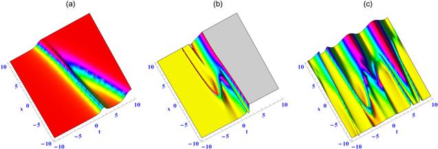
Figure 10. Interaction solution (14) with α1 = η8 = η9 = η10 = α10 = β(t) = 1, α3 = α5 = −1, α2 = 2, y = z = 0, when γ(t) = 1 in (a), γ(t) = t in (b) and $\gamma (t)=\cos t$ in (c). |
4. Interaction solutions between lump and two solitary waves
In order to derive the interaction solutions between lump and two solitary waves, we add two exponential functions in equation (5 ) as follows15 ) into equation (4 ) through Mathematica software, we obtain5 ) and (16 ) into the transformation $u=12\,{[\mathrm{ln}\xi (x,y,z,t)]}_{{xx}}$, we get16 ) is shown in figure 11. Two solitary waves can be found in figure 11(a). A lump wave appears in one of two solitary waves in figure 11(b). In figures 11(c) and 11(d), the lump wave slowly shifts to another solitary wave, until it vanishes in figure 11(e).
$ \begin{eqnarray}\begin{array}{rcl}\zeta & = & x{\alpha }_{1}+y{\alpha }_{2}+z{\alpha }_{3}+{\alpha }_{4}(t),\\ \varsigma & = & x{\alpha }_{5}+y{\alpha }_{6}+z{\alpha }_{7}+{\alpha }_{8}(t),\\ \xi & = & {\zeta }^{2}+{\varsigma }^{2}+{\alpha }_{9}(t)+{\alpha }_{14}(t)\exp [{\alpha }_{13}(t)\\ & & +\ {\alpha }_{10}x+{\alpha }_{11}y+{\alpha }_{12}z]\\ & & +{\alpha }_{15}(t)\exp [-{\alpha }_{13}(t)-{\alpha }_{10}x-{\alpha }_{11}y-{\alpha }_{12}z],\end{array}\end{eqnarray}$
where α15(t) are unknown real functions. Substituting equation ( $ \begin{eqnarray}\begin{array}{rcl}{\alpha }_{6} & = & -\displaystyle \frac{{\alpha }_{1}{\alpha }_{2}}{{\alpha }_{5}},{\alpha }_{7}=-\displaystyle \frac{{\alpha }_{1}{\alpha }_{3}}{{\alpha }_{5}},\\ {\alpha }_{9}(t) & = & \displaystyle \frac{{\alpha }_{10}^{4}{\eta }_{12}+{\alpha }_{1}^{4}+2{\alpha }_{5}^{2}{\alpha }_{1}^{2}+{\alpha }_{5}^{4}}{\left({\alpha }_{1}^{2}+{\alpha }_{5}^{2}\right){\alpha }_{10}^{2}},\\ \varrho (t) & = & \displaystyle \frac{-{\alpha }_{2}^{2}\delta (t)-3{\alpha }_{5}^{2}{\alpha }_{10}^{2}\beta (t)}{{\alpha }_{3}^{2}},\\ {\alpha }_{8}(t) & = & {\eta }_{13}-{\alpha }_{5}\int [3{\alpha }_{10}^{2}\beta (t)+\gamma (t)]\,{\rm{d}}t,\\ {\alpha }_{4}(t) & = & {\eta }_{14}-{\alpha }_{1}\int [3{\alpha }_{10}^{2}\beta (t)+\gamma (t)]\,{\rm{d}}t,{\alpha }_{11}={\alpha }_{12}=0,\\ {\alpha }_{13}(t) & = & {\eta }_{15}-{\alpha }_{10}\int [{\alpha }_{10}^{2}\beta (t)+\gamma (t)]\,{\rm{d}}t\\ & & -\mathrm{ln}{\alpha }_{14}(t),{\alpha }_{15}(t)=\displaystyle \frac{{\eta }_{12}}{{\alpha }_{14}(t)},\end{array}\end{eqnarray}$
with ${\alpha }_{3}\ne 0$, ${\alpha }_{5}\ne 0$, ${\alpha }_{14}(t)\ne 0$, ${\alpha }_{1}^{2}+{\alpha }_{5}^{2}\ne 0$ and ${\alpha }_{10}\ne 0$. Substituting equations ( $ \begin{eqnarray*}\begin{array}{rcl}{u}^{(V)} & = & 12[[2{\alpha }_{1}^{2}+2{\alpha }_{5}^{2}+{\alpha }_{10}^{2}{\alpha }_{14}(t)\exp [{\alpha }_{13}(t)+{\alpha }_{10}x]\\ & & +{\alpha }_{10}^{2}{\alpha }_{15}(t)\exp [-{\alpha }_{10}x\\ & & -{\alpha }_{13}(t)]]/[{\alpha }_{9}(t)+{\alpha }_{14}(t)\exp [{\alpha }_{13}(t)+{\alpha }_{10}x]\\ & & +{\alpha }_{15}(t)\exp [-{\alpha }_{10}x\end{array}\end{eqnarray*}$
$ \begin{eqnarray}\begin{array}{l}-{\alpha }_{13}(t)]+[{\alpha }_{4}(t)+{\alpha }_{1}x+{\alpha }_{2}y+{\alpha }_{3}z]{}^{2}\\ +\left({\alpha }_{8}(t)+{\alpha }_{5}x+{\alpha }_{6}y+{\alpha }_{7}z\right){}^{2}]\\ -[[{\alpha }_{10}{\alpha }_{14}(t)\exp [{\alpha }_{13}(t)+{\alpha }_{10}x]\\ -{\alpha }_{10}{\alpha }_{15}(t)\exp [-{\alpha }_{10}x-{\alpha }_{13}(t)]+2{\alpha }_{1}\\ \ast \ [{\alpha }_{4}(t)+{\alpha }_{1}x+{\alpha }_{2}y+{\alpha }_{3}z]\\ +2{\alpha }_{5}\left({\alpha }_{8}(t)+{\alpha }_{5}x+{\alpha }_{6}y+{\alpha }_{7}z\right)]{}^{2}]/[[{\alpha }_{9}(t)\\ +{\alpha }_{14}(t)\exp [{\alpha }_{13}(t)+{\alpha }_{10}x]\\ +{\alpha }_{15}(t)\exp [-{\alpha }_{10}x-{\alpha }_{13}(t)]+[{\alpha }_{4}(t)\\ +{\alpha }_{1}x+{\alpha }_{2}y+{\alpha }_{3}z]{}^{2}\\ +[{\alpha }_{8}(t)+{\alpha }_{5}x+{\alpha }_{6}y+{\alpha }_{7}z]{}^{2}]{}^{2}]],\end{array}\end{eqnarray}$
where η12, η13, η14 and η15 are integral constants. Interaction phenomena between lump and two solitary waves in equation (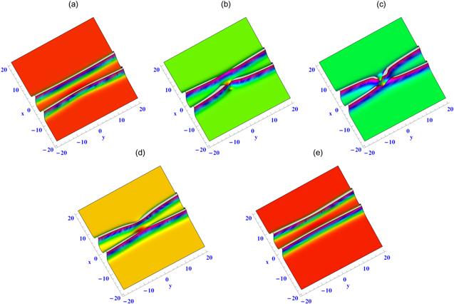
Figure 11. Interaction solution (16) with ${\alpha }_{3}=\gamma (t)=-1$, α2 = α10 = 2, α5 = −3, α1 = η12 = η13 = η14 = η15 = β(t) = 1, z = 0, when t = −1 in (a), t = −0.3 in (b), t = 0 in (c), t = 0.3 in (d), t = 1 in (e). |
5. Conclusion
In this paper, based on the Hirota's bilinear form and Mathematica software [25–35], the lump and interaction solutions between lump and solitary wave of a generalized (3 + 1)-dimensional variable-coefficient nonlinear-wave equation in liquid with gas bubbles are studied. Their physical structures are described in some 3D plots. A periodic-shape rational solution is listed in figure 1(a). A parabolic-shape rational solution is presented in figure 1(b). A cubic-shape rational solution is shown in figure 1(c). In lump solutions (u(II)), the spatial structure called the bright lump wave is seen in figure 2; the spatial structure called the bright-dark lump wave is shown in figure 3. Interaction behaviors of two bright-dark lump waves are presented in figure 4. A periodic-shape bright lump wave is found in figure 5. In lump solutions $({u}^{({III})})$, the spatial structure called the bright lump wave is seen in figure 6. Interaction behaviors of two bright lump waves are presented in figure 7. A periodic-shape bright lump wave is found in figure 8. Figures 9 and 10 display the interaction phenomena between lump and one solitary wave. Figure 11 shows the interaction phenomena between lump and two solitary waves.