In this work, we study the theory of inflation with the non-minimally coupled quadratic, standard model Higgs, and hilltop potentials, through ξφ2R term in Palatini gravity. We first analyze observational parameters of the Palatini quadratic potential as functions of ξ for the high-N scenario. In addition to this, taking into account that the inflaton field φ has a non-zero vacuum expectation value v after inflation, we display observational parameters of well-known symmetry-breaking potentials. The types of potentials considered are the Higgs potential and its generalizations, namely hilltop potentials in the Palatini formalism for the high-N scenario and the low-N scenario. We calculate inflationary parameters for the Palatini Higgs potential as functions of v for different ξ values, where inflaton values are both φ > v and φ < v during inflation, as well as calculating observational parameters of the Palatini Higgs potential in the induced gravity limit for high-N scenario. We illustrate differences between the Higgs potential's effect on ξ versus hilltop potentials, which agree with the observations for the inflaton values for φ < v and ξ, in which v ≪ 1 for both these high and low N scenarios. For each considered potential, we also display ns − r values fitted to the current data given by the Keck Array/BICEP2 and Planck collaborations.
Nilay Bostan. Quadratic, Higgs and hilltop potentials in Palatini gravity[J]. Communications in Theoretical Physics, 2020, 72(8): 085401. DOI: 10.1088/1572-9494/ab7ecb
1. Introduction
Inflation [1–4] is the current accepted model for explaining large scale observations of the universe by positing that there was a period of rapid expansion in the primordial universe. The inflationary big bang model is a solution to main problems in cosmology: isotropy and homogeneity, the spatial flatness, horizon, and unobserved magnetic monopoles. This inflationary era can also produce and extend the small inhomogeneities which have appeared in the large scale structures and the anisotropy in the cosmic microwave background radiation temperature (CMBR). The most recent measurements of the CMBR [5, 6] made by the Planck satellite give some parameters that are related to the inflationary perturbations. Two of these parameters have been measured even more precisely in recent years; the amplitude of the curvature perturbation, ${{\rm{\Delta }}}_{{ \mathcal R }}^{2}\approx 2.4\times {10}^{-9}$ and the corresponding spectral index, ns = 0.9625 ± 0.0048. Another important parameter is the running of the spectral index, α = 0.002 ± 0.010. Even though the constraints on α are not currently sufficient to test the inflationary models, observations of the 21 cm line [7–9] are predicted to improve the measurement of $\alpha ={ \mathcal O }({10}^{-3})$. In addition to this, the recent data from the Keck Array/BICEP2 and Planck collaborations [10] constrains strongly the tensor-to-scalar ratio r < 0.06, which gives a successful explanation to the amplitude of primordial gravitational waves and the scale of inflation. Some ongoing CMB B-mode polarization experiments [11–13] have pushed the limit of r to ≲0.001, or have approached this limit. Each of the parameters above are constrained at the pivot scale of k* = 0.002 Mpc−1.
The observational parameters, in particular the spectral index ns and the tensor-to-scalar ratio r, have been calculated for various inflationary potentials [14]. However, the most minimal realization scenario for the theory of inflation is that the standard model (SM) Higgs boson behaves as the inflaton field with minimal coupling (ξ = 0). On the other hand, a renormalizable scalar field theory in curved space-time needs the non-minimal coupling ξφ2R between the inflaton and the Ricci scalar [15–17]. Furthermore, even if the non-minimal coupling ξ equals to zero at the classical level, it will be created by quantum corrections [15] and in particular, non-minimal coupling to gravity is necessary to sufficiently flatten the Higgs potential at large field values, so that it is in agreement with observations. In this paper we aim to extend the previous studies of how the inflaton field is coupled non-minimally to gravity. We present how the value of the non-minimal coupling parameter ξ affects the observational parameters for the inflationary potentials in the Palatini formalism, in the case of the quadratic potential and symmetry-breaking type inflation potentials where the inflaton field has a non-zero vacuum expectation value v after the period of inflation. A non-zero v after inflation is such that potentials can be related with symmetry-breaking in the very early universe. Examples of such models for symmetry-breaking, which we investigate in this work, are the well-known Higgs inflation [18, 19] models, which are based on the SM of particle physics and especially the Higgs field of the SM behaving as the inflaton field, a scenario first proposed by [19].
In addition to this, [20] has proposed the Lee–Wick SM as an extension of the SM of particle physics supplying an alternative to supersymmetry in terms of addressing the hierarchy problems. They have indicated the cosmology of the Higgs sector of the Lee–Wick SM in order to solve the hierarchy problem. They obtained that homogeneous and isotropic solutions are non-singular, so the Lee–Wick model supplies a possible solution of the cosmological singularity problem. Also, using the Higgs field, many models are taken into account to explain early universe physics, such as bounce inflation. According to this scenario, it is possible to avoid the standard big-bang singularity by adding a non-singular bounce before the inflation period. For instance, [21] has suggested to construct a bounce inflation model with the SM Higgs boson, where the one-loop correction is considered in the effective potential of the Higgs field. According to this model, a Galileon term has been introduced to get rid of the ghost mode when the bounce happens. Finally, we discuss hilltop potentials which are simple generalizations of the Higgs potential.
In this paper, we use dynamics of the Palatini gravity to be able to calculate inflationary parameters. Although the Metric and Palatini formalisms are equivalent in the theory of general relativity, if matter fields are coupled non-minimally to gravity, these two formalisms correspond to two different theories of gravity, as investigated in these [22–27]. In particular, inflationary models with non-minimal couplings to gravity can not be explained with potentials only, gravitational degrees of freedom are required to define such models [22]. The Palatini formalism differs from the Metric formalism in that both the metric gμν and the connection Γ are independent variables. Even though the two formalisms have the same equations of motion, and as a result they correspond to equivalent physical theories, the presence of the non-minimal coupling between gravity and matter causes the physical equivalence to disappear for these two formalisms. In particular the ξ-attractor models which are known as attractor behavior that occurs in the Starobinsky model for larger ξ values in Metric formulation, is lost in the Palatini approach [28] and r can be taken to be much smaller values compared to the Metric formulation for larger ξ values [26, 29–31]. Another important difference between the Metric and Palatini formalism, the inflaton field stays in the sub-Planckian regime to supply a natural inflationary era in the Palatini formalism [22]. In the literature, inflationary potentials in Palatini gravity are taken into account in papers such as these [22, 24, 25, 32–34]. In [24] the quadratic potential is discussed in Palatini gravity taking N* = 50 and N* = 60, they found that the strength of the non-minimal coupling, $\xi ={ \mathcal O }({10}^{-3})$ agrees with the current data just for N* = 60. In addition to this, Higgs inflation in the Palatini formulation has been studied in [22, 25, 32–34]. According to these papers, predictions of r are very tiny for ξ ≳ 1 values and so r is suppressed further leading to well-known attractor behavior in the Starobinsky model of the Metric formulation for large ξ values, whereas the attractor behavior vanishes in the Palatini approach.
This paper is organized as follows, we first describe inflation with a non-minimal coupling and how inflationary parameters are calculated (section 2) in the Palatini formulation. Next, we analyze the Palatini quadratic potential in the large-field limit for the high N scenario (section 3). We then calculate inflationary predictions in detail for two different symmetry-breaking inflation type potentials (Higgs potentials) (section 4) for inflaton values φ > v and φ < v. We then illustrate that hilltop potentials can be compatible with the current measurements for cases of φ < v and ξ, v ≪ 1 (section 5). Furthermore, (in section 4) we calculate inflationary parameters in the induced gravity limit for Palatini Higgs inflation. Finally, we discuss our results and summarize them (section 6).
2. Palatini inflation with a non-minimal coupling
We describe a non-minimally coupled scalar field φ with a canonical kinetic term and a potential VJ(φ). Then the inflation action in the Jordan frame becomes
In the metric formulation, the connection is taken as a function of the metric tensor. It is called the Levi-Civita connection $\bar{{\rm{\Gamma }}}=\bar{{\rm{\Gamma }}}({g}^{\mu \nu })$
On the other hand, in the Palatini formalism both gμν and Γ are independent variables, and the only assumption here is that the connection is torsion-free, i.e. ${{\rm{\Gamma }}}_{\mu \nu }^{\lambda }={{\rm{\Gamma }}}_{\nu \mu }^{\lambda }$. By solving equations of motion, one can obtain the following [22]
in the Palatini formulation. In this work, in order to calculate inflationary parameters of symmetry-breaking type inflation potentials, we choose the F(φ) to include a constant m2 term and a non-minimal coupling ξφ2R, which is necessary for a renormalizable scalar field theory in curved space-time [15–17] as we mentioned above. We are using units, where the reduced Planck scale ${m}_{{\rm{P}}}=1/\sqrt{8\pi G}\approx 2.4\times {10}^{18}\ \mathrm{GeV}$ is set equal to unity. Thus, either F(φ) → 1 or φ → 0 is required after inflation. In that case, by taking m2 = 1 − ξv2 into consideration, we obtain F(φ) = m2 + ξφ2 = 1 + ξ(φ2−v2) [35]. Furthermore, we take Palatini quadratic potential in the large-field limit into account. So, to be able to compute observational parameters, we take F(φ) = 1 + ξφ2.
2.1. Calculating the inflationary parameters
The difference between Metric and Palatini formulations are more easily figured out in the Einstein frame. By applying a Weyl rescaling gE,μν = gμν/F(φ), we can show the Einstein frame action in the form
we obtain the action for a minimally coupled scalar field χ with a canonical kinetic term. Using equation (2.7), Einstein frame action in terms of χ can be obtained in the form
For F(φ) = 1 + ξ(φ2−v2), different limit cases for equation (2.6) can be obtained:
1. Electroweak regime
If $| \xi ({\phi }^{2}-{v}^{2})| \ll 1$, φ ≈ χ and VJ(φ) ≈ VE(χ). Thus, in this limit, the inflationary predictions for the non-minimal coupling case are approximately the same with the ones for the minimal coupling case.
in the Palatini formulation. Using equation (2.10), inflationary potential can be taken into account in terms of canonical scalar field χ, therefore slow-roll parameters are written for Palatini formulation in the large-field limit according to χ.
On the condition that Einstein frame potential is written in terms of the canonical scalar field χ, inflationary parameters can be found using the slow-roll parameters [37]
where the subscript ‘*' indicates quantities when the scale corresponding to k* exited the horizon, and χe is the inflaton value at the end of inflation, which we obtain by ε(χe) = 1.
The amplitude of the curvature perturbation in terms of canonical scalar field χ is written the form
The best fit value for the pivot scale k* = 0.002 Mpc−1 is ${{\rm{\Delta }}}_{{ \mathcal R }}^{2}\approx 2.4\times {10}^{-9}$ [5] from the Planck results. Furthermore, we redefine the slow-roll parameters in terms of the scalar field φ for numerical calculations, because for all general ξ and v values, it is not possible to compute the inflationary potential in terms of χ. Using equations (2.7) and (2.11) together, slow-roll parameters can be found in terms of φ [38]
To compute the values of inflationary parameters, we should obtain a value for N* numerically. Under the assumption of a standard thermal history after inflation, N* is given as follows [39]
here, ρe = (3/2)V(φe) is the energy density at the end of inflation, ρ* ≈ V(φ*) is the energy density when the scale corresponding to k* exited the horizon, ρr is the energy density at the end of reheating and ωr is the equation of state parameter throughout reheating, which we take its value to be constant. Predictions of the inflationary parameters change depending on the total number of e-folds.
2.2. Different reheating scenarios
In literature, most of the papers take N* ≈ 50–60 as a constant while calculating the inflationary parameters in general. On the other hand, to be able to discriminate inflationary models from each other, their predictions should be more accurate. Therefore, to indicate an acceptable range of N* depending upon reheating temperature, we take three different scenarios into account to define N*:
1. High-N scenario
ωr = 1/3, this case corresponds to the assumption of instant reheating.
2. Middle-N scenario
ωr = 0 and the temperature of reheating is taken as Tr = 109 GeV, while computing ρr using the SM value for the usual number of relativistic degrees of freedom values for g* = 106.75.
3. Low-N scenario
ωr = 0, same as middle-N scenario. But in this case, the reheat temperature Tr = 100 GeV.
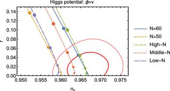
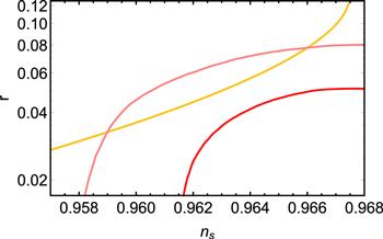
The ns − r curves for different scenarios are displayed in figure 1 for the Higgs potential in the Palatini formulation (debated in section 4) together with the 68% and 95% confidence level (CL) contours based on the data taken by the Keck Array/BICEP2 and Planck collaborations [10]. The figure illustrates the curves for the confidential N* values of 50 and 60, which are necessarily taken in agreement with the range expected from a standard thermal history after inflation for the Higgs potential in the Palatini formalism. However, N* is smaller (for example between roughly 45–55 providing that v ∼ 0.01) for the hilltop inflation models (described in section 5), because inflation takes place at a lower energy scale in these models.
Figure 1. The figure illustrates that ns − r predictions for different ξ values and v = 0.01 for various reheating cases as described in the text for Higgs potential in the Palatini formalism. The points on each curve represent ξ = 10−2.5, 10−2, 10−1.5, 10−1, and 1, top to bottom. The pink (red) contour corresponds to the 95% (68%) CL contours based on the data taken by the Keck Array/BICEP2 and Planck collaborations [10].
3. Quadratic potential
The quadratic inflation potential model in Jordan frame is given by in the form
here, m is a mass term. By using equation (2.14) and the value of amplitude for the curvature power spectrum ${{\rm{\Delta }}}_{{ \mathcal R }}^{2}\approx 2.4\,\times {10}^{-9}$, we can fix the required mass to be m ≃ 6 × 10⁻⁶ for N = 60 and minimal coupling case, thus ns ≃ 0.967 and r ≃ 0.16. The results are slightly disfavored by the latest observational data [10].
In the large-field limit (described in section 2), Einstein frame quadratic potential for Palatini approach in terms of χ using equation (2.10) can be obtained as follows
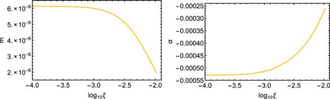
As it can be seen from equation (3.2), by expanding this potential around the minimum for large ξ values, we can obtain the flattening potential. In literature [24], analyzed the values of ns, r and m for the quadratic potential in Palatini gravity taking N* = 50 and N* = 60 to be constant. In this work, we analyze ns, r, α and m values as a function of ξ for the Palatini quadratic potential with large-field limit numerically for the high-N scenario. According to our results from figure 2, we find that if the non-minimal coupling parameter between the range 10−4 ≲ ξ ≲ 10−3 for the high-N scenario, values of ns can be inside the observational region, and as it can be seen from figure 3, m ≃ 6 × 10⁻⁶ for the range of 10−4 ≲ ξ ≲ 10−3. However, for the ξ ≃ 10−2 value, m ≃ 2 × 10⁻⁶. As a result, the energy scale should be determined by the observational values on the amplitude on the scalar power spectrum.
Figure 2. The figure shows that ns − r predictions for quadratic potential in the Palatini formalism for high-N scenario for the different ξ values that are mentioned in the text. The pink (red) contour correspond to the 95% (68%) CL contour given by the Keck Array/BICEP2 and Planck collaborations [10].
Figure 3. For quadratic potential in the Palatini formalism for high-N scenario, the figures show that m and α values as functions of ξ.
In the case of larger ξ, ns values decrease and they remain outside the observational region. For the range between 10−4 ≲ ξ ≲ 10−2, we obtain 0.01 ≲ r ≲ 0.12. Furthermore, for the low-N scenario, inflationary parameters of Palatini quadratic potential remain the outside the observational region for any ξ value. Finally, figure 3 shows that α values are very tiny for this type of potential.
4. Higgs potential
In this section, we take a well-known symmetry-breaking type potential into account [40]
which is known as the Higgs potential. This potential was investigated for the minimal coupling case in such recent papers, see [14, 41–44]. In this case, when inflation takes place around the minimum, the potential is approximately quadratic and thus the quadratic potential predictions in terms of N*
can be obtained for inflation both φ > v and φ < v. In this work, instead of minimal coupling case, we analyze the Higgs inflation with non-minimal coupling in Palatini formulation both high-N scenario and low-N scenario. Furthermore, using equation (2.17), we obtain N* for non-minimally coupled Palatini Higgs inflation analytically in the form
In the large-field limit (described in section 2), for Palatini Higgs inflation with non-minimal coupling, ns, r and α can be found using equation (2.7) together with equations (2.10), (2.12) and (2.13) in terms of N*
On the other hand, in the case of φ ≪ v when cosmological scales exit the horizon, the potential approximates to the hilltop potential type (described as section 5), effectively
Predictions of this potential type in equation (4.5) for φ ≪ v that r is very suppressed and ns ≈ 1–8/v2. In this section, we analyze numerically for φ > v and φ < v cases in the high-N scenario and the low-N scenario for Higgs potential with non-minimal coupling in the Palatini approach with broad range of ξ and v. In literature, inflationary predictions of Palatini Higgs inflation were taken into account for different N* values, in general taken to be constant between N* ≈ 50–60 [33, 34, 45–47]. For example, [33] analyzed the preheating stage following the end of Palatini Higgs inflation by taking N* ≈ 50. They showed that the slow decaying oscillations of Higgs afterwards the end of inflation, permits the field to periodically return to the plateau of the potential so the preheating stage in the Palatini Higgs inflation is necessarily instantaneous. Therefore, this decrease in N* is required to solve the problems of hot big bang.
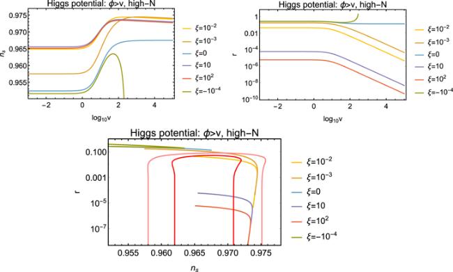
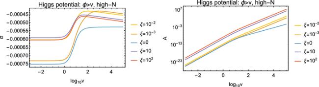
First of all, we illustrate φ > v case for both scenarios. As it can be seen in figures 4 and 5, ξ ≤ 0 cases are outside the 95% CL contour given by Keck Array/BICEP2 and Planck collaborations [10] for all v values. In addition to this, for small v values, inflationary predictions of ξ = 10−3 can be outside the 95% CL contour. However, in larger v values, predictions are inside 95% CL for ξ = 10−3. For ξ = 10−2, predictions are inside 68% CL for small v values but for larger values of v, predictions remain within 95% CL contour. Furthermore, for ξ ≫ 1 cases, predictions are inside 68% CL for small values of v and when v increases, they enter in the 95% CL and r is very tiny for larger and smaller values of v, so r is highly suppressed at any v values for larger ξ cases. For ξ = 10−2 and ξ = 10−3, r is very small for large v values but this case is not valid for smaller values of v. For both ξ < 0 and ξ = 0 cases, r does not take very small values for larger and smaller v. In addition to this, as it can be seen that from figure 5, α takes very tiny values to be observed in the near future observations for selected ξ cases and at any v values. Moreover, for all selected ξ values, when v increases, values of A increase depending on v.
Figure 4. For Higgs potential in the Palatini formalism in the cases of φ > v and high-N scenario, in the top figures display changing ns and r values for different ξ cases as function of v and the bottom figure shows that ns − r predictions for selected ξ values. The pink (red) contour correspond to the 95% (68%) CL contour given by the Keck Array/BICEP2 and Planck collaborations [10].
Figure 5. For Higgs potential in the Palatini formalism, the change in α and A as a function of v is plotted for different ξ values in the cases of φ > v and high-N scenario.
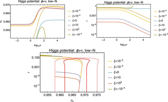
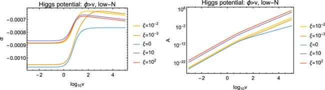
In addition to φ > v and high-N cases, figures 6 and 7 illustrate the φ > v but low-N case for the Higgs potential in the Palatini formalism. According to figure 6, predictions of ξ = 0 and ξ < 0 cases are similar to φ > v and high-N scenario results. On the other hand, predictions for the remaining ξ values slightly differ from the high-N case. For ξ ≫ 1 cases, predictions can be in the 95% CL contour for small v values but when v increases, predictions remain inside 68% CL. In the low-N case, values of r for all the selected ξ values overlap with the high-N case, so again r is very small for ξ ≫ 1 cases for both small and large v values. Also for larger values of v for ξ = 10−2 and ξ = 10−3 cases, r is also very tiny except for small v values. Furthermore, in the low-N case, values of α and A are similar to the high-N case, so α takes very small values for our selected ξ cases and for all v values to be observed in the near future measurements.
Figure 6. For Higgs potential in the Palatini formalism in the cases of φ > v and low-N scenario, in the top figures display changing ns and r values for different ξ cases as function of v and the bottom figure shows that ns − r predictions for selected ξ values. The pink (red) contour correspond to the 95% (68%) CL contour given by the Keck Array/BICEP2 and Planck collaborations [10].
Figure 7. For Higgs potential in the Palatini formalism, the change in α and A as a function of v is plotted for different ξ values in the cases of φ > v and low-N scenario.
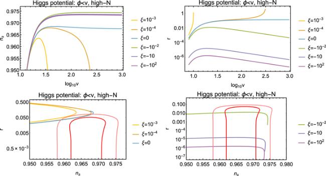
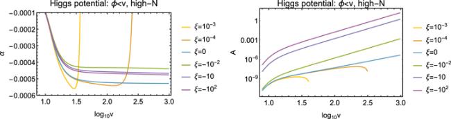
Numerical results for φ < v and high-N cases for Higgs potential in the Palatini approach can be seen in figures 8 and 9. According to these figures, predictions of ξ = 10−3 are ruled out for current data. In contrast, ξ = 10−4 and ξ = 0 cases can be inside the 95% CL contour given by the Keck Array/BICEP2 and Planck collaborations [10]. However, ξ < 0 cases for the range between 10 ≲ v ≲ 20, predictions are outside the 95% CL contour, but when v increases, they can be in the region compatible with observational data depending on v. Unlike from φ > v and high-N scenario, here the values of r are very small for ξ = −10 and ξ = −102 cases. In addition to this, α values are very small similar to other situations. Lastly, for ξ ≤ 0 cases, values of A increase depending on v, but this case is different for ξ = 10−3 and ξ = 10−4 values, as it can be seen in figure 9.
Figure 8. For Higgs potential in the Palatini formalism in the cases of φ < v and high-N scenario, in the top figures display changing ns and r values for different ξ cases as function of v. The bottom figures show that ns − r predictions for selected ξ values, left panel: ξ > 0 and ξ = 0 cases, right panel: ξ < 0 cases. The pink (red) contour correspond to the 95% (68%) CL contour given by the Keck Array/BICEP2 and Planck collaborations [10].
Figure 9. For Higgs potential in the Palatini formalism, the change in α and A as a function of v is plotted for different ξ values in the cases of φ < v and high-N scenario.
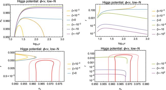
Furthermore, we also obtain numerical results in the cases of φ < v and low-N scenario for the Higgs potential in figures 10 and 11. According to these figures, inflationary predictions of ξ ≥ 0 cases are ruled out for current data. In addition to this, the cases of ξ < 0, predictions begin to enter the observational region, when v increases. For larger v values, predictions remain inside the 68% CL contour, as well as the values of r are strongly suppressed for cases of both ξ = −10 and ξ = −102. According to figure 11, results for the α and A are the same as φ < v and high-N scenario. We also display inflationary parameters of the Higgs potential in the limit of induced gravity, described as in the text (see section 2) for high-N scenario in figure 12. According to this figure, all our selected ξ values are in the 68% CL contour. What is more, in this limit case, α values are also very tiny for all v and values of A increase, depending upon v.
Figure 10. For Higgs potential in the Palatini formalism in the cases of φ < v and low-N scenario, in the top figures display changing ns and r values for different ξ cases as function of v. The bottom figures show that ns − r predictions for selected ξ values, left panel: ξ > 0 and ξ = 0 cases, right panel: ξ < 0 cases. The pink (red) contour correspond to the 95% (68%) CL contour given by the Keck Array/BICEP2 and Planck collaborations [10].
Figure 11. For Higgs potential in the Palatini formalism, the change in α and A as a function of v is plotted for different ξ values in the cases of φ < v and low-N scenario.
Figure 12. For Higgs potential in the Palatini formalism, the change in ns, r, α and A as a function of v is plotted for different ξ values and for φ > v in the induced gravity limit which corresponds to ξv2 = 1.
In the induced gravity limit, using equation (2.9), the Einstein frame potential can be obtained in terms of χ in the form
For this potential, using equation (2.13), 8ξN ≈ $\exp \left(2\sqrt{\xi }\chi \right)$. Therefore, using equation (2.12) we can find ns and r approximately in the induced gravity limit
The Higgs potential in the induced gravity limit was previously investigated for the Metric formulation in [48–50]. In this work, we extend these papers by analyzing the Higgs potential in the induced gravity limit in the Palatini formulation for φ > v and high-N scenario. To sum up, in literature, Higgs inflation with non-minimal coupling has been discussed such [35, 38, 48–51] in the Metric formulation. References [38] and (for just ξ > 0) [51] analyzed the Higgs inflation with non-minimal coupling in the Metric formulation in general by taking F(φ) = 1 + ξφ2. Moreover, [35] explained the Higgs inflation with non-minimal coupling in the Metric formulation for both ξ > 0 and ξ < 0 cases for F(φ) = 1 + ξ(φ2−v2). On the other hand, some papers took non-minimally coupled Higgs inflation in the Palatini formulation into account [22, 25, 32, 33], which we mentioned before. Reference [22] examined for the large-field limit by taking F(φ) = 1 + ξφ2 and they found ns ≃ 0.968 and r ≃ 10−14 in the Palatini approach. In addition to this, by taking F(φ) = 1 + ξφ2, [25] found predictions of various inflationary parameters in the Palatini approach. They also found that r values are highly suppressed for ξφ2 ≫ 1 limits and they obtained very small α values to be observed in the future measurements. Similar to the other papers [33], analyzed Palatini Higgs inflation by taking F(φ) = 1 + ξφ2. Different from previous papers, we analyze inflationary parameters of the Palatini Higgs inflation with non-minimal coupling using F(φ) = m2 + ξφ2 = 1 + ξ (φ2−v2). Furthermore, we display our numerical calculations using both the high-N and the low-N scenario.
5. Hilltop potentials
In this section, we take other symmetry-breaking type potential models into account which also take place in some supersymmetric inflation models, i.e. [52–54] for the case of the inflaton value is φ < v throughout inflation. These potential types can be described with the generalization of the Higgs potential in the form
In the electroweak regime, which explained in section 2, we have φ ≈ χ and also χ ≪ v during inflation, and the Einstein frame potential can be obtained as in terms of canonical scalar field
where we have defined τ = v/21/μ. In the literature, hilltop potentials with minimal coupling case (ξ = 0) have been investigated such [14, 37]. Furthermore, by taking the equations (2.11)–(2.13) into consideration, we find
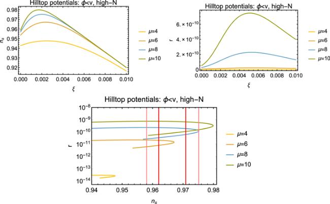
which illustrates that r is strongly suppressed and ns takes smaller values than the range in agreement with observational results. On the other hand in this work, we calculate inflationary parameters for hilltop potentials with non-minimal coupling in Palatini formulation, both for the high-N and the low-N scenario numerically. The results of these calculations are shown in figures 13–16. Furthermore, for the potential in equation (5.2), ns and r can be obtained in the form
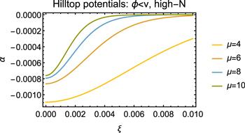
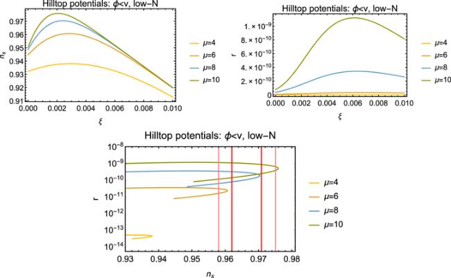
These predictions are compatible with our numerical results for ns − r that were computed using the Jordan frame potential described by equation (5.1) which is shown in the top figures in the figures 13 and 15 for two different scenarios. As it can be seen from the figures 13–16 in general, on the condition that ξ, v ≪ 1 and τ = 0.01, observational parameters can be inside observational region except for μ = 4 since predictions are ruled out for any ξ values in the case of μ = 4 for both scenarios which we take into account. In addition to this, as the ξ values increase, observational parameters are ruled out for any ξ values in the cases of μ = 6, 8, 10 different from smaller ξ values as well as r values are highly suppressed and also values of α are very tiny to be observed in the near future measurements for all selected μ values.
Figure 13. For hilltop potentials in the Palatini formalism, top figures display that ns, r values as functions of ξ for τ = 0.01 and different μ values in the cases of φ < v and high-N scenario. The bottom figure displays ns − r predictions based on range of the top figures ξ values for τ = 0.01. The pink (red) line corresponds to the 95% (68%) CL contour given by the Keck Array/BICEP2 and Planck collaborations [10].
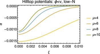
Figure 14. For hilltop potentials in the Palatini formalism, the figure shows that α values as functions of ξ for τ = 0.01 and different μ values in the cases of φ < v and high-N scenario.
Figure 15. For hilltop potentials in the Palatini formalism, top figures display that ns, r values as functions of ξ for τ = 0.01 and different μ values in the cases of φ < v and low-N scenario. The bottom figure displays ns − r predictions based on range of the top figures ξ values for τ = 0.01. The pink (red) line corresponds to the 95% (68%) CL contour given by the Keck Array/BICEP2 and Planck collaborations [10].
Figure 16. For hilltop potentials in the Palatini formalism, the figure shows that α values as functions of ξ for τ = 0.01 and different μ values in the cases of φ < v and low-N scenario.
6. Conclusion
In this work, we briefly expressed the Palatini inflation with a non-minimal coupling in section 2. Considering non-minimally coupled scalar fields, we discussed how these two formalisms differ from each other in section 2. A very important feature is the that Palatini approach ensures a natural inflation since the inflaton in this formalism remains below the Planckian regime. The other thing is that like strong suppression of tensor perturbations, form additional distinctive features of the Palatini approach compared to the Metric one.
We displayed our results for the inflationary predictions of non-minimally coupled Palatini quadratic potential in the large-field limit for high-N scenario in section 3 for F(φ) = 1 + ξφ2. Next, we analyzed the predictions of the Higgs potential for φ > v and φ < v in section 4 and hilltop potentials for φ < v in section 5 with non-minimal coupling in the Palatini formulation by taking F(φ) = 1 + ξ(φ2−v2) for both N scenarios. Furthermore, in section 4, we also investigated the Higgs potential in the induced gravity limit for the high-N scenario.
We illustrated that for the Palatini quadratic potential with non-minimal coupling, only small ξ values fit the current measurements given by the Keck Array/BICEP2 and Planck collaborations [10] for the high-N case. According to our results, r has very tiny values in the ξ ≫ 1 cases where the inflaton value φ > v for the Higgs potential for the high-N scenario and the low-N scenario. Therefore, we found that the significant Starobinsky attractor behavior for larger ξ values in the Metric formulation disappears in the Palatini formulation for these ξ cases where the inflaton value φ > v for both two scenarios. In addition to this, for ξ = 10−2 and ξ = 10−3, r has very tiny values solely for larger v. However, in the case of φ < v and for also both scenarios, r values are highly suppressed for ξ = −10 and ξ = −102.
We also analyzed the Palatini Higgs inflation in the induced gravity limit for the high-N scenario and we found that for ξ ≥ 1 cases, r takes small values. Furthermore, we calculated the inflationary predictions of hilltop potentials numerically in the case of the inflaton value φ < v and ξ, v ≪ 1 for the high-N scenario and the low-N scenario. In these types of potentials, inflationary parameters can be compatible with approximately ξ ≲ 0.005 values just in the cases of φ < v and v ≪ 1. We also obtained that r values are highly suppressed in the hilltop potentials for both scenarios.
In general, we conclude that a non-minimally coupled scalar field in the Palatini approach gives a plausible inflationary evolution for the early universe. Last but not least, we obtained that the prediction of α is too small to be observed in future measurements for all our examined potentials but we consider that more enhanced values of α could be provided by experiments in the near future, observations of the 21 cm line in particular [7–9].
LindeA D1982 A new inflationary universe scenario: a possible solution of the horizon, flatness, homogeneity, isotropy and primordial monopole problems Phys. Lett. B108 389
KohriKOyamaYSekiguchiTTakahashiT2013 Precise measurements of primordial power spectrum with, 21cm fluctuations J. Cosmol. Astropart. Phys.2013 JCAP10(2013)065
BasseTHamannJHannestadSWongY Y Y2015 Getting leverage on inflation with a large photometric redshift survey J. Cosmol. Astropart. Phys.2015 JCAP06(2015)042
AdeP A R (BICEP2 and Keck Array Collaborations) 1810 BICEP2/Keck array x: constraints on primordial gravitational waves using planck, WMAP, and new BICEP2/Keck observations through the, 2015 season Phys. Rev. Lett.121 221301
CaiY FQiuT TBrandenbergerRZhangX M2009 A nonsingular cosmology with a scale-invariant spectrum of cosmological perturbations from Lee–Wick theory Phys. Rev. D80 023511
BostanNGüleryüzÖŞenoğuzV N2018 Inflationary predictions of double-well, Coleman–Weinberg, and hilltop potentials with non-minimal coupling J. Cosmol. Astropart. Phys.2018 JCAP05(2018)046
LythD HLiddleA R2009The Primordial Density Perturbation: Cosmology, Inflation and the Origin of Structure Cambridge Cambridge University Press
38
LindeANoorbalaMWestphalA2011 Observational consequences of chaotic inflation with nonminimal coupling to gravity J. Cosmol. Astropart. Phys.2011 JCAP03(2011)013
DestriCde VegaH JSanchezN G2008 MCMC analysis of WMAP3 and SDSS data points to broken symmetry inflaton potentials and provides a lower bound on the tensor to scalar ratio Phys. Rev. D77 043509


