


1. Introduction
Motivated by the outcome originating from the investigation of black hole thermodynamics [1, 2], Hooft [3] proposed the holographic principle (principle of quantum gravity) that all of the evidence enclosed in a volume of space can be characterized as a hologram, which relates to a theory locating on the boundary of that space. Earlier, Susskind [4] presented a specific string-hypothesis which clarified this principle. Moreover, Maldacena [5] gives the best acknowledgment of the holographic principle from its well-known AdS/CFT correspondence. Observational evidence from a type-Ia supernova (SNe-Ia) suggests the Universe is increasing at an accelerating rate [6], which suggests the existence of dark energy with negative pressure and positive energy density fulfilling the conditions of the equation of state. After the sudden discovery of dark energy [6, 7], it has ended up being one of the crucial issues in theoretical physics and the current cosmology. Also, the present observations support a cosmological constant Λ being the source of dark energy driving the present accelerated epoch of the Universe. This cosmological model is called the ΛCDM model. Despite the fact that it is favored by the observations, the ΛCDM model experiences constant cosmological problems [8–11]. To overcome this, various dark energy models have been proposed. It is accepted that the dark energy issue might be an issue of quantum gravity. Accordingly, holographic principle may play an important role in solving the dark energy issue. By applying the holographic principle to dark energy Li et al [12] anticipated the holographic dark energy model in which the IR cut-off is favored as the size of things to come with the event horizon of the Universe. This makes holographic dark energy a very competitive candidate of dark energy. The holographic dark energy can derive an accelerating expansion of the Universe and is in great concurrence with the present cosmological observation. As of late, the world view of holographic dark energy has drawn a lot of deception and has been widely considered. The generalized holographic dark energy models have been observed in the investigation of Jamil et al [13]. Sarkar [14] investigated a holographic dark energy model with linearly varying deceleration parameters and a generalized Chaplygin gas dark energy model for a Bianchi type-I Universe, whereas Banerjee and Roy [15] presented the stability of a holographic dark energy model. Pasqua et al [16] and Sing and Srivastava [17] studied the consequences of three modified types of holographic dark energy models in Bulk–Brane connection with viscous cosmology in a new holographic dark energy model and cosmic acceleration, respectively.
A choice to represent the current accelerating cosmic expansion is the modification in the Einstein gravity. The f(R) theory of gravity [18] gives a characteristic unification of the early-time inflation and late-time acceleration together with the natural gravitational attraction in contrast to dark energy. Likewise, this theory covers all the domains from the cosmological to the nearby planetary scales [19]. A few prominent authors given in [20–30] have studied f(R) gravity for various space-times in the different contexts of use. Due to the occurrence of torsion without introducing dark energy, an accelerated expansion of the Universe is seen in teleparallel gravity, specifically f(T) gravity. Several authors [31–41] have explored a few highlights of cosmological models within the framework of f(T) gravity.
In view of cosmic acceleration, energy conditions (all the more viably strong energy condition) is the subject of much discussion as the strong energy condition is violated on a cosmological scale of cosmic acceleration [42]. The violation of this condition exhibits a transition from being attractive to repulsive, which is just like the behavior of dark energy for cosmic acceleration. Alongside these conditions are extensively exploited as basic tools not only for the Hawking–Penrose singularity theorems, but for the validity of the second regulation of black hole thermodynamics [43]. In [44] is the proof, no longer solely for an integral connection between gravitation and black hole thermodynamics, but horizon entropy and the vicinity of a black hole. Additionally, the generalized second law of thermodynamics is an energizing topic in an accelerating Universe which has been thought of widely. Exploiting the Hawking temperature together with Bekenstein entropy Wang et al [45] found that the laws of thermodynamics are not valid at the event horizon. Henceforth, the Universe bounded by the event horizon is not a perfect thermodynamic system, while modification of the Hawking temperature is an ideal thermodynamic framework [46]. Many authors [47–56] have examined thermodynamics at the evident horizon with the Hawking temperature. As a situation for good compatibility with observational data and to describe the accelerated expansion of the Universe, some contemporary models of teleparallel gravity, in which torsion, the traces of the matter, energy–momentum tensor and boundary term are addressed, are presented in [57–59]. Specifically, f(T, B) gravity has a better advantage because one recovers the same formation in both scenarios of f(T) and f(R) gravity. It is a great option in contrast to dark energy, which is brought about by the consistency of teleparallel-curvature, and is thus called f(R, T) gravity. Subsequently, f(T, B) gravity attracts more attention from researchers.
Encouraged by the above discussions and outcomes, in this article we have explored the type of holographic dark energy called the Tsallis holographic dark energy model in f(T, B) gravity by validating the second law of thermodynamics in the model. In this paper, we talk about vitality conditions for the isotropic homogeneous Friedman–Lemâitre–Robertson–Walker (FLRW) Universe model with a perfect fluid matter source in f(T, B) gravity. The paper is presented as follows: in section 2 , we formulate the field equations in f(T, B) gravity relating the Tsallis holographic dark energy source. Section 3 investigates field equations corresponding to the FLRW Universe. In section 4 , we derive the solution of the field equation which corresponds to an accelerated expansion. In section 5 , the dynamical parameters and their physical discussions are presented. Physical acceptability and stability of the model utilizing the speed of sound, energy conditions and validity of the generalized second law of thermodynamics are given in section 6 , while section 7 contains the concluding remarks.
2. The ${\boldsymbol{f}}({\boldsymbol{T}},{\boldsymbol{B}})$ gravity and Tsallis holographic dark energy
Consider the action for the combination of f(R) and f(T) gravity, namely f(T, B) gravity [59], as follows
$ \begin{eqnarray}S=\int e\left(\displaystyle \frac{f(T,B)}{{\kappa }^{2}}+{L}_{m}\right){{\rm{d}}}^{4}x,\end{eqnarray}$
where ${\kappa }^{2}=8\pi G$ and f(T, B) is a function of the torsion scalar T and the boundary term $B=\tfrac{2}{e}{\partial }_{\mu }({{eT}}^{\mu })$ in which ${T}_{\mu }={T}_{v\mu }^{\mu }$. Lm and $e=\det ({e}_{\mu }^{i})$ are the matter action and determinant of tetrad components, respectively.By varying the action given in equation (1 ) with respect to the tetrad, the field equation is defined as
$ \begin{eqnarray}\begin{array}{l}2e{\delta }_{\nu }^{\lambda }{{\rm{\nabla }}}^{\mu }{{\rm{\nabla }}}_{\mu }{\partial }_{B}f-2e{{\rm{\nabla }}}^{\lambda }{{\rm{\nabla }}}_{\nu }{\partial }_{B}f+{eB}{\partial }_{B}f{\delta }_{\nu }^{\lambda }\\ \quad +\,4e\left({\partial }_{\mu }{\partial }_{B}f+{\partial }_{\mu }{\partial }_{T}f\right){S}_{\nu }^{\mu \lambda }+4{e}_{\nu }^{a}{\partial }_{\mu }\left({{eS}}_{a}^{\mu \lambda }\right){\partial }_{T}f\\ \quad -\,4e{\partial }_{{Tf}}{T}^{\sigma }{}_{\mu \nu }{S}_{a}^{\lambda \mu }-{ef}{\delta }_{\nu }^{\lambda }=16\pi {{eT}}_{\nu }^{\lambda }.\end{array}\end{eqnarray}$
As we know, in the standard cosmological model, the Universe is well thought out by a perfect fluid. Therefore, the energy–momentum tensor for perfect fluid is written as $ \begin{eqnarray}{T}_{v}^{\lambda }=(\rho +p){u}_{v}{u}^{\lambda }-p{\delta }_{v}^{\lambda },\end{eqnarray}$
where ρ and p are the energy density and the pressure of the fluid inside the Universe, respectively. Here, ${u}^{\nu }\,=\left(0,0,0,1\right)$ with ${u}^{\nu }{u}_{\nu }=1$ are the comoving coordinates, where ${u}^{\nu }$ is the four-velocity vector of the fluid. The non-zero element of the energy–momentum tensor is given by $ \begin{eqnarray}{T}_{0}{}^{0}=\rho ,{T}_{1}{}^{1}={T}_{2x}{}^{2}={T}_{3}{}^{3}=-p.\end{eqnarray}$
Considering quantum corrections for the holographic dark energy model, Tsallis and Cirto showed the black hole horizon entropy as [50] $ \begin{eqnarray}{S}_{\delta }={\gamma }_{1}{A}^{\delta },\end{eqnarray}$
where γ1 is a constant, and δ refers to a positive non-additive parameter. By setting δ = 1 and ${\gamma }_{1}=\tfrac{1}{4G}$ the Bekenstein entropy is effectively recouped [60].In [61] Cohen et al reproduced the holographic dark energy in view of vacuum energy whose furthest cut-off esteem is not well beyond the dark energy. Following the above supposition one can accomplish the connection between the framework entropy S, IR cut-off L and UV(Λ) cut-offs as5 ) and (6 ), one can find
$ \begin{eqnarray}{L}^{3}{{\rm{\Lambda }}}^{3}\leqslant {S}^{3/4}.\end{eqnarray}$
Combing equations ( $ \begin{eqnarray}{{\rm{\Lambda }}}^{4}\leqslant {\gamma }_{1}{\left(4\pi \right)}^{\delta }{L}^{2\delta -4},\end{eqnarray}$
where Λ4 represents the vacuum energy density.In addition, expending the above equations (6 ) and (7 ) Tavayef et al [60] proposed new a holographic dark energy model, the so-called Tsallis holographic dark energy density of the form8 ) as
$ \begin{eqnarray}{\rho }_{{\rm{THDE}}}={ \mathcal B }{L}^{2\delta -4},\end{eqnarray}$
where ${ \mathcal B }$ is an unknown parameter. The IR cut-off as the Hubble horizon is given by $ \begin{eqnarray}L=\displaystyle \frac{1}{H}.\end{eqnarray}$
Using the above equation, we can get the Tsallis holographic dark energy density from ( $ \begin{eqnarray}{\rho }_{{\rm{THDE}}}={ \mathcal B }{H}^{4-2\delta }.\end{eqnarray}$
3. Metric and components of field equations
We consider the spatially homogeneous and isotropic FLRW line element in the form
$ \begin{eqnarray}{\rm{d}}{s}^{2}={\rm{d}}{t}^{2}-{a}^{2}(t)\left[\displaystyle \frac{{\rm{d}}{r}^{2}}{1-{{kr}}^{2}}+{r}^{2}{\rm{d}}{\theta }^{2}+{r}^{2}{\sin }^{2}\theta \ {\rm{d}}{\phi }^{2}\right],\end{eqnarray}$
where a is the scale factor of the Universe, and $(t,\ r,\ \theta ,\ \phi )$ are the comoving coordinates.The angle $\theta $ and φ are the the standard azimuthal and polar edges of circular directions, with $0\leqslant \theta \leqslant \pi $ and $0\leqslant \phi \leqslant 2\pi $. The homogeneity of the Universe fixes a unique edge of reference. Additionally, k is the constant describing the curvature of the space. Here, k = 1 describes a closed Universe, the flat Universe is acquired for k = 0 and k = −1 relates to an open Universe. In this work, we consider the flat Universe taking k = 0 with endless range.
The equation of motion (2 ) for the spatially homogeneous and isotropic FLRW line element (11 ) with the fluid of the stress–energy tensor (4 ) can be written as
$ \begin{eqnarray}-3{H}^{2}(3\partial {}_{B}f+2{\partial }_{T}f)+3H{\partial }_{B}\dot{f}-3\dot{H}{\partial }_{B}f+\displaystyle \frac{1}{2}f={\kappa }^{2}\rho ,\end{eqnarray}$
$ \begin{eqnarray}\begin{array}{l}-(3{H}^{2}+\dot{H})(3{\partial }_{B}f+2{\partial }_{T}f)\\ \quad -\,2H{\partial }_{T}\dot{f}+{\partial }_{B}\ddot{f}+\displaystyle \frac{1}{2}f=-{\kappa }^{2}p.\end{array}\end{eqnarray}$
The overhead dot represents the differentiation with respect to cosmic time t.The torsion scalar for the metric (11 ) is written as11 ) is obtained as15 ) is found as
$ \begin{eqnarray}T=-6{H}^{2}.\end{eqnarray}$
The torsion scalar and Ricci scalar are related together as $ \begin{eqnarray}R=-T+B.\end{eqnarray}$
All the standard activity in relativity carried out is made with the Ricci scalar R; however, in f(T, B) gravity it is made with the torsion scalar T alongside the boundary term B. This issue discloses to us that these models are distinctive just by the limit (boundary) term [59]. The limit term for the metric ( $ \begin{eqnarray}B=-6\left(\dot{H}+3{H}^{2}\right).\end{eqnarray}$
The Ricci scalar R from ( $ \begin{eqnarray*}R=-6\left(\dot{H}+2{H}^{2}\right).\end{eqnarray*}$
However, the standard forms of Friedman equations are of the form $ \begin{eqnarray}3{H}^{2}={\kappa }^{2}{\rho }_{{\rm{tot}}},\end{eqnarray}$
$ \begin{eqnarray}2\dot{H}+3{H}^{2}=-{\kappa }^{2}{\bar{p}}_{{\rm{tot}}}.\end{eqnarray}$
As the Universe is overwhelmed by another fluid other than an ideal fluid in f(T, B) gravity, the parameters ${\rho }_{{\rm{tot}}}$ and ${p}_{{\rm{tot}}}$ are written as follows: $ \begin{eqnarray}{\rho }_{{\rm{tot}}}=\rho +{\rho }_{d},\end{eqnarray}$
$ \begin{eqnarray}{p}_{{\rm{tot}}}=p+{p}_{d}.\end{eqnarray}$
Recently, considering two cases of a non-interacting and interacting fluid scenario Aditya et al [62] investigated the dark energy phenomenon by studying the Tsallis holographic dark energy within the framework of the Brans–Dicke scalar tensor theory of gravity (where the Brans–Dicke scalar field is a logarithmic function of the scale factor a(t) and Hubble's horizon as the IR cut-off).Using equations (12 ), (13 ), (17 )–(20 ), we find ρd and pd as21 ) and (22 ) are slightly different from those of the equations presented in (12 ) and (13 ) in view of the standard Friedman equations provided in (17 ) and (18 ). Hence, we consider that equations (21 ) and (22 ) are the density and pressure of dark energy for f(T, B) gravity. Here, we have considered $f\,=f(T,B)=\alpha {T}^{m}+\beta {B}^{n}$.
$ \begin{eqnarray}{\kappa }^{2}{\rho }_{d}=3{H}^{2}(1+3{\partial }_{B}f+2{\partial }_{T}f)-3H{\partial }_{B}\dot{f}+3\dot{H}{\partial }_{B}f-\displaystyle \frac{1}{2}f,\end{eqnarray}$
$ \begin{eqnarray}\begin{array}{rcl}{\kappa }^{2}{p}_{d} & = & -3{H}^{2}(1+3{\partial }_{B}f+2{\partial }_{T}f)-\dot{H}(2+3{\partial }_{B}f+2{\partial }_{T}f)\\ & & -2H{\partial }_{T}\dot{f}+{\partial }_{B}\ddot{f}+\displaystyle \frac{1}{2}f,\end{array}\end{eqnarray}$
where the quantities ${\rho }_{d}$ and pd are the parts of the energy density and pressure, respectively, appearing from f(T, B) gravity, and these are representative of dark energy. The expressions of ρd and pd presented in equations (The measurements with red-shift data for supernovae from SNe-Ia have led to the prediction of an accelerating as well as flat Universe with ${\rm{\Omega }}={{\rm{\Omega }}}_{{\rm{m}}}+{{\rm{\Omega }}}_{{\rm{d}}}=1$, where the values Ωm = 0.3, Ωd = 0.7. This value of the density parameter Ωd corresponds to a cosmological constant that is very small, but nevertheless, non-zero and positive. The components of the total energy density parameter Ω, such as the energy densities for dark energy Ωd and matter Ωm, are given as [63]
$ \begin{eqnarray}{{\rm{\Omega }}}_{{\rm{d}}}=\displaystyle \frac{{\rho }_{d}}{\rho {}_{c\tau }}=\displaystyle \frac{{\rho }_{d}}{3{H}^{2}},\end{eqnarray}$
$ \begin{eqnarray}{{\rm{\Omega }}}_{{\rm{m}}}=\displaystyle \frac{\rho }{{\rho }_{c\tau }}=\displaystyle \frac{\rho }{3{H}^{2}},\end{eqnarray}$
where ${\rho }_{c\tau }$ is the critical energy density of the Universe.4. Explication of isotropic homogeneous space-time
The most striking revolution of the modern cosmology (type-Ia supernovae) is a consensus on the conclusion that the Universe has entered a state of accelerating expansion at red shift $z\sim -0.5$ with the range of deceleration parameter $-1\leqslant q\leqslant 0$ (the exact value is q = −0.45). The law of variation for the Hubble's parameter was initially proposed by Bermann and Gomide [64] because FLRW space-time yields a constant value of the deceleration parameter, and later it was valid for the time-varying deceleration parameter [65]. After the discovery of the late-time acceleration of the Universe, many authors have used the constant deceleration parameter to obtain cosmological models in the context of dark energy within the general theory of relativity and also modified theories of gravity. The deceleration parameter is defined as
$ \begin{eqnarray}q=-\displaystyle \frac{a\ddot{a}}{{\dot{a}}^{2}}.\end{eqnarray}$
The sign q indicates whether the model accelerates or decelerates. The negative sign q indicates acceleration, whereas a positive value stands for deceleration. Also, recent observations of SNe-Ia reveal that the present Universe is accelerating for H > 0 and q < 0. In this article, we use the well-known relation between the Hubble parameter H and scale factor a [66] as $ \begin{eqnarray}H={{ba}}^{-\eta },\end{eqnarray}$
where b > 0 and η ≥ 0 are constants. The above relation yields a constant deceleration parameter.Using the definition of the Hubble parameter $H=\tfrac{\dot{a}}{a}$, we can get27 ) yields
$ \begin{eqnarray}\dot{a}={{ba}}^{-\eta +1},\end{eqnarray}$
$ \begin{eqnarray}\ddot{a}=-{b}^{2}(\eta -1){a}^{-2\eta +1}.\end{eqnarray}$
Consequently, the deceleration parameter q takes the form $ \begin{eqnarray}q=-1+\eta ,\end{eqnarray}$
which is a constant. Integration of equation ( $ \begin{eqnarray}a={\left(\eta {bt}+{b}_{1}\right)}^{\tfrac{1}{\eta }}={\left({a}_{1}t+{b}_{1}\right)}^{\gamma },\end{eqnarray}$
provided $\gamma =\tfrac{1}{\eta }=\tfrac{1}{1+q}$, where $q\ne -1$ and ${a}_{1}=\eta b\ne 0$, b1 are constants of integration.From equation (30 ), it is observed that the scale factor of the model is the function of cosmic time, which increases with time at q > −1, decreases with time at q < −1 and does not exist at q = −1.
5. Dynamical parameters and their physical discussion
The dynamical parameters like spatial volume, the Hubble parameter and scalar expansion have the following expressions.
The spatial volume of the metric is
$ \begin{eqnarray}V=a{}^{3}={\left({a}_{1}t+{b}_{1}\right)}^{3\gamma }.\end{eqnarray}$
The Hubble parameter is $ \begin{eqnarray}H=\displaystyle \frac{\gamma {a}_{1}}{{a}_{1}t+{b}_{1}}.\end{eqnarray}$
The scalar expansion is $ \begin{eqnarray}\theta =3H=\displaystyle \frac{3\gamma {a}_{1}}{{a}_{1}t+{b}_{1}}.\end{eqnarray}$
In our investigation, it is found that the spatial volume V and the scale factor a of the Universe are built up with a constant value at $t\to 0$, and with the expansion of cosmic time they are consistently growing; when $t\to \infty $ the spatial volume V and $\ a\to \infty $. This shows the model starts with constant volume at $t\to 0$ and expands with infinite time (see figure 1). Additionally, the scalar expansion and the Hubble parameter are both consistent throughout the expansion of the Universe, which shows that the Universe is expanding with the expansion of cosmic time; however, the rate of expansion decreases to a steady worth, which shows that the Universe begins to evolve with constant volume at $t\to 0$ with the infinite rate of expansion.
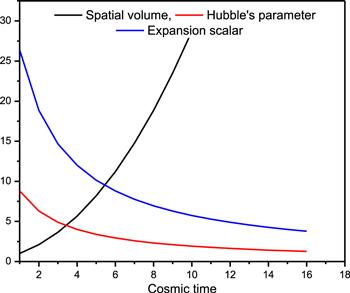
Figure 1. Spatial volume, the Hubble parameter and scalar expansion versus cosmic time for the appropriate choice of constants: a1 = 4, b1 = 1 and γ = 2.2. |
The graphical behavior of the Tsallis holographic dark energy density (which is obtained from equation (10 ) together with the value of the Hubble parameter given in equation (32 )) versus cosmic time for the appropriate choice of constants, a1 = 4, b1 = 1 and γ = 2.2, is well-defined in figure 2 towards 0 ≤ δ ≤ 2, out of which for δ = 1.0 the Tsallis holographic dark energy density reduces to holographic dark energy density.
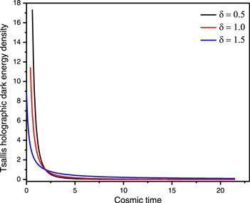
Figure 2. Tsallis holographic dark energy density versus cosmic time for the appropriate choice of constants: a1 = 4, b1 = 1, δ = 0.5, 1.0, 1.5 and γ = 2.2. |
The expressions of dark energy density and pressure from equations (21 ) and (22 ) are obtained as
$ \begin{eqnarray}\begin{array}{rcl}{\rho }_{d} & = & \displaystyle \frac{3{a}_{1}^{2}{\gamma }^{2}}{{\left({a}_{1}t+{b}_{1}\right)}^{2}}+\displaystyle \frac{(3m\alpha \gamma -2{m}^{2}\alpha +m\alpha -3\alpha \gamma +\alpha ){a}_{2}}{3(\gamma -1){\left({a}_{1}t+{b}_{1}\right)}^{2m}}\\ & & -\displaystyle \frac{\beta (2n+1){b}_{2}}{2{\left({a}_{1}t+{b}_{1}\right)}^{2n}}+\displaystyle \frac{18m\alpha {a}_{1}^{3}\gamma {a}_{2}}{{\left({a}_{1}t+{b}_{1}\right)}^{2m+3}},\end{array}\end{eqnarray}$
and $ \begin{eqnarray}\begin{array}{rcl}{p}_{d} & = & \displaystyle \frac{{a}_{1}^{2}\gamma (1-3\gamma )}{{\left({a}_{1}t+{b}_{1}\right)}^{2}}+\displaystyle \frac{{a}_{3}}{\gamma (3\gamma -1){\left({a}_{1}t+{b}_{1}\right)}^{2m}}\\ & & +\displaystyle \frac{{b}_{3}}{3\gamma {\left({a}_{1}t+{b}_{1}\right)}^{2n}}\\ & & -\displaystyle \frac{12n\beta {a}_{1}^{3}\gamma {b}_{2}}{{\left({a}_{1}t+{b}_{1}\right)}^{2n+3}}+\displaystyle \frac{\alpha {{ma}}_{2}}{2{a}_{1}\gamma (3\gamma -1){\left({a}_{1}t+{b}_{1}\right)}^{2m-1}},\end{array}\end{eqnarray}$
where ${a}_{2}={[6{a}_{1}^{2}\gamma (3\gamma -1)]}^{m}$, ${b}_{2}={[-6{a}_{1}^{2}{\gamma }^{2}]}^{n}$, ${a}_{3}\,=\tfrac{3}{2}m{\gamma }^{2}{a}_{2}+\tfrac{1}{2}m\alpha \gamma {a}_{2}+\tfrac{3}{2}{m}^{2}(m-1)\alpha {a}_{2}+\tfrac{1}{2}\gamma (3\gamma -1)$ and ${b}_{3}=3n\beta \gamma {b}_{2}-n\beta {b}_{2}-2n(n-1)\gamma {b}_{2}$ + $\tfrac{3}{2}\beta \gamma {b}_{2}$.It is seen that the dark energy density is consistently non-negative and a decreasing function of cosmic time (see figure 3), while the pressure is initially positive and, with the expansion, it becomes negative (figure 4). In the beginning, when $t\to 0$ the Universe has a constant energy density and pressure, whereas when $t\to \infty $ the energy density ${\rho }_{d}\to 0$ and pressure pd < 0. It is interesting to take note that the dark energy density acquired in equation (8 ) obtained in general relativity and the component of the dark energy density obtained from $f\left(T,B\right)$ gravity presented in equation (34 ) are both exhibiting the same behavior (in relation to inverse cosmic time) just for the selection of constants, i.e. $\delta ={ \mathcal B }=1$.

Figure 3. The behavior of dark energy density versus cosmic time t for the appropriate choice of constants: a1 = 4, b1 = 1, α = 0.1, β = 36, m = 1, n = 1 and γ = 2.2. |

Figure 4. The behavior of dark energy pressure versus cosmic time t for the appropriate choice of constants: a1 = 4, b1 = 1, α = 0.1, β = 36, m = 1, n = 1 and γ = 2.2. |
From equations (33 ) and (34 ), the expression of the dark energy equation of state parameter is obtained as
$ \begin{eqnarray}\begin{array}{l}{\omega }_{d}=\displaystyle \frac{\left(\tfrac{{a}_{1}^{2}\gamma (1-3\gamma )}{{\left({a}_{1}t+{b}_{1}\right)}^{2}}+\tfrac{{a}_{3}}{\gamma (3\gamma -1){\left({a}_{1}t+{b}_{1}\right)}^{2m}}+\tfrac{{b}_{3}}{3\gamma {\left({a}_{1}t+{b}_{1}\right)}^{2n}}-\tfrac{12n\beta {a}_{1}^{3}\gamma {b}_{2}}{{\left({a}_{1}t+{b}_{1}\right)}^{2n+3}}+\tfrac{\alpha {{ma}}_{2}}{2{a}_{1}\gamma (3\gamma -1){\left({a}_{1}t+{b}_{1}\right)}^{2m-1}}\right)}{\left(\tfrac{3{a}_{1}^{2}{\gamma }^{2}}{{\left({a}_{1}t+{b}_{1}\right)}^{2}}+\tfrac{(3m\alpha \gamma -2{m}^{2}\alpha +m\alpha -3\alpha \gamma +\alpha ){a}_{2}}{3(\gamma -1){\left({a}_{1}t+{b}_{1}\right)}^{2m}}-\tfrac{\beta (2n+1){b}_{2}}{2{\left({a}_{1}t+{b}_{1}\right)}^{2n}}+\tfrac{18m\alpha {a}_{1}^{3}\gamma {a}_{2}}{{\left({a}_{1}t+{b}_{1}\right)}^{2m+3}}\right)}.\end{array}\end{eqnarray}$
Equation (36 ) represents the equation state parameter of dark energy, which is depicted in figure 5. The outcomes originating from SNe-Ia information together with cosmic microwave background radiation anisotropy and galaxy clustering statistics yield ωd = −0.97 (Wilkinson Microwave Anisotropy Probe, SNe-Ia results) at a 68% certainty level of dark energy. These outcomes are reliable with the time-variable equation of state parameter ωd(t) and, furthermore, for the time-free ωd. On the underlying stage, when the Universe began to grow for a slight interval of cosmic time, the equation of state parameter had the value ωd > 0, i.e. the model behaved like matter dominated once at the beginning, while with expansion it differs and varies from the quintessence region (ωd > −1) at a later time with the value −0.9 ∼ −0.97. Henceforth, at a later time, the model shows a quintessence model and remains present in the same quintessence dominated region at infinite expansion of the model, which bears some similarity to the hypothetical outcomes originating from SNe-Ia information together with cosmic microwave background radiation anisotropy and galaxy clustering statistics.

Figure 5. The dark energy equation of state parameter versus cosmic time for the appropriate choice of constants: a1 = 4, b1 = 1, α = 0.1, β = 36, m = 1, n = 1 and γ = 2.2. |
From equations (23 ) and (24 ), the components of the total energy density parameter, such as energy densities of dark energy and dark matter, are obtained as37 ) and (38 ), the total energy density parameter takes the form
$ \begin{eqnarray}\begin{array}{rcl}{{\rm{\Omega }}}_{{\rm{d}}} & = & \displaystyle \frac{{a}_{1}^{2}\gamma }{{\alpha }^{2}}+\displaystyle \frac{(3m\alpha \gamma -2{m}^{2}\alpha +m\alpha -3\alpha \gamma +\alpha ){a}_{2}}{9{\gamma }^{2}{\alpha }^{2}(\gamma -1){\left({a}_{1}t+{b}_{1}\right)}^{2m-2}}\\ & & -\displaystyle \frac{\beta (2n+1){b}_{2}}{{\gamma }^{2}{\alpha }^{2}6{\left({a}_{1}t+{b}_{1}\right)}^{2n-2}}+\displaystyle \frac{6{{ma}}_{1}^{3}{a}_{2}}{\gamma \alpha {\left({a}_{1}t+{b}_{1}\right)}^{2m+1}},\end{array}\end{eqnarray}$
$ \begin{eqnarray}\begin{array}{rcl}{{\rm{\Omega }}}_{{\rm{m}}} & = & 1-\displaystyle \frac{{a}_{1}^{2}\gamma }{{\alpha }^{2}}-\displaystyle \frac{(3m\alpha \gamma -2{m}^{2}\alpha +m\alpha -3\alpha \gamma +\alpha ){a}_{2}}{9{\gamma }^{2}{\alpha }^{2}(\gamma -1){\left({a}_{1}t+{b}_{1}\right)}^{2m-2}}\\ & & +\displaystyle \frac{\beta (2n+1){b}_{2}}{{\gamma }^{2}{\alpha }^{2}6{\left({a}_{1}t+{b}_{1}\right)}^{2n-2}}-\displaystyle \frac{6{{ma}}_{1}^{3}{a}_{2}}{\gamma \alpha {\left({a}_{1}t+{b}_{1}\right)}^{2m+1}}.\end{array}\end{eqnarray}$
Using equations ( $ \begin{eqnarray}{\rm{\Omega }}={{\rm{\Omega }}}_{{\rm{d}}}+{{\rm{\Omega }}}_{{\rm{m}}}=1.\end{eqnarray}$
One can see from the above equation that the total energy density parameter is equal to 1, which recommends that the model is flat.6. Physical acceptability and stability of solutions
6.1. Stability of the model
For the stability of the corresponding solution in the present model, we should check the physical acceptance. For this, firstly it is required that the velocity of sound should be less than the velocity of light, i.e. within the range $0\lt {\vartheta }_{s}^{2}=\tfrac{\partial p}{\partial \rho }$. For the present model, we obtained the velocity of sound speed as
$ \begin{eqnarray}{\vartheta }_{s}^{2}=\displaystyle \frac{\left(-\tfrac{{a}_{1}^{3}\gamma (1-3\gamma )}{{\left({a}_{1}t+{b}_{1}\right)}^{3}}-\tfrac{2{{ma}}_{1}{a}_{3}}{\gamma (3\gamma -1){\left({a}_{1}t+{b}_{1}\right)}^{2m+1}}+\tfrac{2{{na}}_{1}{b}_{3}}{3\gamma {\left({a}_{1}t+{b}_{1}\right)}^{2n+1}}-\tfrac{12n\beta {a}_{1}^{4}\gamma {b}_{2}(2n+3)}{{\left({a}_{1}t+{b}_{1}\right)}^{2n+4}}+\tfrac{\alpha {{ma}}_{2}(1-2m)}{2\gamma (3\gamma -1){\left({a}_{1}t+{b}_{1}\right)}^{2m}}\right)}{\left(-\tfrac{6{a}_{1}^{3}{\gamma }^{2}}{{\left({a}_{1}t+{b}_{1}\right)}^{3}}+\tfrac{2{{ma}}_{1}(3m\alpha \gamma -2{m}^{2}\alpha +m\alpha -3\alpha \gamma +\alpha ){a}_{2}}{3(\gamma -1){\left({a}_{1}t+{b}_{1}\right)}^{2m+1}}+\tfrac{n\beta {a}_{1}(2n+1){b}_{2}}{{\left({a}_{1}t+{b}_{1}\right)}^{2n+1}}-\tfrac{18m\alpha {a}_{1}^{4}\gamma {a}_{2}(2m+3)}{{\left({a}_{1}t+{b}_{1}\right)}^{2m+4}}\right)}.\end{eqnarray}$
Figure 6, shows that at the initial epoch ${\vartheta }_{s}^{2}\gt 0$, and with the expansion ${\vartheta }_{s}^{2}\lt 0$. Hence, the model is initially stable, but with expansion it is unstable.
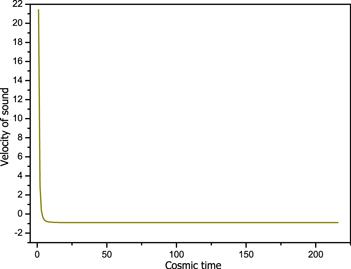
Figure 6. The stability factor (velocity of sound) of the dark energy model versus cosmic time for the appropriate choice of constants: a1 = 4, b1 = 1, α = 0.1, β = 36, m = 1, n = 1 and γ = 2.2. |
6.2. Energy conditions
In this section, we are going to discuss the various energy conditions, which are linear combinations of the energy density and pressure. The various energy conditions available in the literature are namely the weak energy condition (WEC), strong energy condition (SEC), null energy condition (NEC) and dominant energy condition (DEC) [67–70]. Since ‘normal' matter speaks to positive energy density and pressure, thus conventional-issue will naturally fulfill the NEC, WEC and SEC. In this investigation, we should emphasize the energy conditions for the components of dark energy which come out from f(T, B) gravity. The different types of energy conditions are defined as:
| i | (i) WEC: ${\rho }_{d}\geqslant 0$, ${\rho }_{d}+{p}_{d}\geqslant 0$. |
| ii | (ii) SEC: ${\rho }_{d}+3{p}_{d}\geqslant 0$. |
| iii | (iii) NEC: ${\rho }_{d}+{p}_{d}\geqslant 0$. |
| iv | (iv) DEC: ${\rho }_{d}-\left|{p}_{d}\right|\geqslant 0$. |
The energy density of the Universe is positive with the evolution. The expansion of positive energy density in the NEC yields the WEC. The condition of time like the killing vector results in the SEC, whose violation describes the accelerating expansion of the Universe [68]. The singularity theorems by Hawking–Penrose require the validity of both the WEC and SEC. The NEC and WEC are very important among all energy conditions as the remaining energy conditions violate due to the transition from being attractive to repulsive, which is just like the behavior of dark energy for cosmic acceleration.
Our investigation of current observations suggests that the WEC, NEC and DEC are all fulfilled (see figures 3, 7, 9) through the expansion of the Universe, while the SEC is validated in figure 8 at some point as the epoch of galaxy formation (initially) and then violated. Specifically, the classical singularity theorem that is significant in demonstrating the presence of the huge explosion utilizes the SEC [43]. The plots of ρd and ${\rho }_{d}+{p}_{d}$ versus cosmic time appear in the panels of figures 3 and 7. We see that pd represents positive decreasing behavior initially for a small interval of cosmic time, and with expansion it becomes negative and remains present as pd < 0 for a whole range of cosmic time. The plot of ρd along the cosmic time is positive when decreasing and approximately constant but remains positive. The plot of ${\rho }_{d}+{p}_{d}$ versus cosmic time represents decreasing behavior with respect to t. However, the plot indicates a positive value of ${\rho }_{d}+{p}_{d}$ throughout the expansion of the model. Thus, the WEC is also satisfied for our derived model.
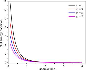
Figure 7. The behavior of the NEC, ${\rho }_{d}+{p}_{d}\geqslant 0$ in the dark energy model versus cosmic time for the appropriate choice of constants: a1 = 4, b1 = 1, α = 0.1, β = 36, m = 1, 3, 5, 7, n = 1 and γ = 2.2. |
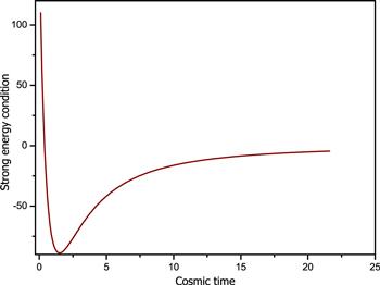
Figure 8. The behavior of the SEC, ${\rho }_{d}+3{p}_{d}\geqslant 0$ versus cosmic time with the appropriate choice of constants: a1 = 4, b1 = 1, α = 0.1, β = 36, m = 1, n = 1 and γ = 2.2. |

Figure 9. The behavior of the DEC, ${\rho }_{d}-\left|{p}_{d}\right|\geqslant 0$ versus cosmic time with the appropriate choice of constants: a1 = 4, b1 = 1, α = 0.1, β = 36, m = 1, n = 1 and γ = 2.2. |
6.3. Validity of generalized second law of thermodynamics at the horizon
Here, we have examined the validity of the generalized thermodynamics second law of the f (T, B) theory of gravity. The energy–momentum tensor of additional geometric components satisfies the following conservation equation [71]41 ) the energy conservation equation is not satisfied if $2{\dot{f}}_{T}\ne 0$. We can find the radius of the dynamical apparent horizon for the flat FLRW space-time as17 ) and (18 ) gives43 ) and (44 ), we get45 ), we have42 ) and (49 ), the Misner–Sharp energy turns out to be17 ) and (49 ) one can find48 ) and (51 ), we get52 ), with the help of the above equation, can be written as55 ) can be revamped as55 ) and (58 ), the required condition for validity of the generalized second law of thermodynamics is written as
$ \begin{eqnarray}{\rho }_{d}=3H({\rho }_{d}+{p}_{d})=\displaystyle \frac{T}{2{\kappa }^{2}}(2{\dot{f}}_{T}).\end{eqnarray}$
From equation ( $ \begin{eqnarray}{\tilde{r}}_{A}=\displaystyle \frac{1}{H}.\end{eqnarray}$
The time derivative of the above equation together with equations ( $ \begin{eqnarray}\displaystyle \frac{{f}_{T}{\rm{d}}{\tilde{r}}_{A}}{2\pi G}=-{\tilde{r}}_{A}^{3}H({p}_{{\rm{tot}}}+{\rho }_{{\rm{tot}}}){\rm{d}}t.\end{eqnarray}$
In general relativity and f(R) gravity the Bekenstein–Hawking horizon entropy is defined as ${S}_{h}=\tfrac{A}{4G}$, where $A=4\pi {\tilde{r}}_{A}^{2}$ is the area of the apparent horizon [44] and ${S}_{h}=\tfrac{A}{4{G}_{{\rm{tot}}}}$, where ${G}_{{\rm{tot}}}=\tfrac{G}{{f}_{R}}$, which is associated with the Noether charge, the so-called Wald entropy [44]. Similarly, f(T) gravity is defined as ${S}_{h}=\tfrac{A}{4{G}_{{\rm{tot}}}}$, where ${G}_{{\rm{tot}}}=\tfrac{G}{{f}_{T}}$ [72]. In the f(T, B) gravity theory the Wald entropy is defined as [73] $ \begin{eqnarray}{S}_{h}=-\displaystyle \frac{A(2{f}_{T})}{4G}.\end{eqnarray}$
From equations ( $ \begin{eqnarray}\displaystyle \frac{{\rm{d}}{S}_{h}}{2\pi {\tilde{r}}_{A}}=\displaystyle \frac{{\tilde{r}}_{A}(-{\rm{d}}{f}_{T})}{G}+4\pi {\tilde{r}}_{A}^{3}H(p+\rho ){\rm{d}}t.\end{eqnarray}$
The associated temperature of the apparent horizon through the surface gravity ${\kappa }_{{\rm{sg}}}$ is defined as [73] $ \begin{eqnarray}{\tilde{T}}_{H}=\displaystyle \frac{\left|{\kappa }_{{\rm{sg}}}\right|}{2\pi },\end{eqnarray}$
where ${\kappa }_{{\rm{sg}}}$ is given by $ \begin{eqnarray}{\kappa }_{{\rm{sg}}}=-\displaystyle \frac{{\tilde{r}}_{A}}{2}(2{H}^{2}+\dot{H}).\end{eqnarray}$
From multiplication of $\left(1-\tfrac{{\dot{\tilde{r}}}_{A}}{2H{\tilde{r}}_{A}}\right)$ on both sides of equation ( $ \begin{eqnarray}\begin{array}{rcl}{\tilde{T}}_{H}{\rm{d}}{S}_{h} & = & 4\pi {\tilde{r}}_{A}^{3}H({p}_{{\rm{tot}}}+{\rho }_{{\rm{tot}}}){\rm{d}}t\\ & & -2\pi {\tilde{r}}_{A}^{2}H({p}_{{\rm{tot}}}+{\rho }_{{\rm{tot}}}){\rm{d}}{\tilde{r}}_{A}-\displaystyle \frac{\pi {\tilde{r}}_{A}^{2}{\tilde{T}}_{H}{\rm{d}}(2{f}_{T}){\rm{d}}t}{G}.\end{array}\end{eqnarray}$
In general relativity, the Misner–Sharp energy is defined as $E=\left(\tfrac{{\tilde{r}}_{A}}{2G}\right)$, whereas in f(T, B) gravity, this definition can be extended as [73] $ \begin{eqnarray}E=-\displaystyle \frac{{\tilde{r}}_{A}(2{f}_{T})}{2G}.\end{eqnarray}$
From equations ( $ \begin{eqnarray}E=-{ \mathcal V }\displaystyle \frac{3{H}^{2}(2{f}_{T})}{2G}={ \mathcal V }{\rho }_{{\rm{tot}}},\end{eqnarray}$
where ${ \mathcal V }=\left(4/3\right)\pi {\tilde{r}}_{A}$ is known as the volume of the interior region of the apparent horizon. From equations ( $ \begin{eqnarray}{\rm{d}}E=-\displaystyle \frac{{\tilde{r}}_{A}}{G}{\rm{d}}{f}_{T}+4\pi {\rho }_{{\rm{tot}}}{\tilde{r}}^{2}{\rm{d}}{\tilde{r}}_{A}-4\pi H{\tilde{r}}^{3}{}_{A}({\rho }_{{\rm{tot}}}+{p}_{{\rm{tot}}}){\rm{d}}t.\end{eqnarray}$
Using equation ( $ \begin{eqnarray}\begin{array}{rcl}{\tilde{T}}_{H}{\rm{d}}{S}_{h} & = & -{\rm{d}}E+2\pi {\tilde{r}}^{2}{}_{A}({\rho }_{{\rm{tot}}}-{p}_{{\rm{tot}}}){\rm{d}}{\tilde{r}}_{A}\\ & & -\displaystyle \frac{{\tilde{r}}_{A}}{G}(2\pi {\tilde{r}}_{A}{\tilde{T}}_{H}+1){\rm{d}}{f}_{T}.\end{array}\end{eqnarray}$
The work density is obtained as $ \begin{eqnarray}W=-\displaystyle \frac{1}{2}\left({\hat{T}}^{\left(m\right)\alpha \beta }{h}_{\alpha \beta }+{\hat{T}}^{\left(d\right)\alpha \beta }{h}_{\alpha \beta }\right)=\displaystyle \frac{1}{2}\left({\rho }_{{\rm{tot}}}-{p}_{{\rm{tot}}}\right).\end{eqnarray}$
Equation ( $ \begin{eqnarray}{\tilde{T}}_{H}{\rm{d}}{S}_{h}=-{\rm{d}}E+W{\rm{d}}{ \mathcal V }-\displaystyle \frac{{\tilde{r}}_{A}}{G}\left(2\pi {\tilde{r}}_{A}{\tilde{T}}_{H}+1\right){\rm{d}}{f}_{T},\end{eqnarray}$
which takes the form $ \begin{eqnarray}{\tilde{T}}_{H}{\rm{d}}{S}_{h}+{\tilde{T}}_{H}{\rm{d}}\tilde{S}=-{\rm{d}}E+W{\rm{d}}{ \mathcal V }.\end{eqnarray}$
In the above condition the term ${\rm{d}}{\tilde{S}}_{h}=\tfrac{{\tilde{r}}_{A}}{G{\tilde{T}}_{H}}\left(2\pi {\tilde{r}}_{A}{\tilde{T}}_{H}+1\right){\rm{d}}{f}_{T}$ can be treated as an entropy creation in a non-balanced (equilibrium) thermodynamic framework because of the Lagrangian depending upon both the torsion scalar and the boundary term [73]. The f(T) gravity includes just T, while f(T, B) gravity includes both the torsion and boundary terms. In f(T, B) gravity ${\rm{d}}\tilde{S}\ne 0$, due to $2{\rm{d}}{f}_{T}\ne 0$. Here, we may characterize the compelling entropy term as being the total of the horizon entropy and the entropy generation term as ${S}_{{\rm{tot}}}={S}_{h}+\bar{S}$, with the goal that equation ( $ \begin{eqnarray}{\tilde{T}}_{H}{\rm{d}}{S}_{{\rm{tot}}}=-{\rm{d}}E+W{\rm{d}}{ \mathcal V }.\end{eqnarray}$
To examine the second law of thermodynamics in f(T, B) modified gravity, one needs to consider the Gibbs equation in terms of dark energy and matter components as $ \begin{eqnarray}{\tilde{T}}_{{\rm{tot}}}{\rm{d}}{S}_{t}={\rm{d}}({\rho }_{{\rm{tot}}}{ \mathcal V })+{p}_{{\rm{tot}}}{\rm{d}}{ \mathcal V }={ \mathcal V }{\rm{d}}({\rho }_{{\rm{tot}}})+({\rho }_{{\rm{tot}}}+{p}_{{\rm{tot}}}){\rm{d}}{ \mathcal V },\end{eqnarray}$
where ${S}_{{\rm{tot}}}$ stands for the total entropy of the system inside the horizon. Here, we assume that the relation between the total temperature of the energy source inside the horizon and to the temperature of the apparent horizon as ${\tilde{T}}_{{\rm{tot}}}=\varepsilon {\tilde{T}}_{h}$, where $0\lt \varepsilon \lt 1$. The authenticity of the generalized second law of thermodynamics needs the condition $ \begin{eqnarray}\displaystyle \frac{{\rm{d}}{S}_{h}}{{\rm{d}}t}+\displaystyle \frac{{\rm{d}}({\rm{d}}\bar{S})}{{\rm{d}}t}+\displaystyle \frac{{\rm{d}}{S}_{{\rm{tot}}}}{{\rm{d}}t}\geqslant 0.\end{eqnarray}$
Using the FLRW equation along with equations ( $ \begin{eqnarray}\displaystyle \frac{{f}_{T}}{{{GH}}^{2}}\left\{\left(2-\varepsilon \right)-2\left(1-\varepsilon \right)(2\dot{H}-H)\right\}\geqslant 0.\end{eqnarray}$
Pourbagher and Amani [71] investigated the accelerated expansion of the Universe by investigating the stability of the model using the sound speed parameter along with the validity of the generalized second law of thermodynamics in the f(T, B) theory of gravity. Bahamonde et al [73] studied different features of a flat FLRW cosmology and showed that the FLRW equations can be transformed into the form of the Clausius relation, which contains contributions both from horizon entropy and an additional entropy term introduced due to the non-equilibrium, and formulated the constraint for the validity of the generalized second law of thermodynamics.
The derived result shows that the validity of the generalized second law of thermodynamics is satisfied with conditions of thermodynamic equilibrium. This issue is pressing in that the temperatures of the Universe outside and inside of the apparent horizon are either similar or different. Hence, by applying the thermodynamic equilibrium condition, the generalized second law of thermodynamics for the dark energy in the f(T, B) gravity model in a flat FLRW Universe with an apparent horizon is validated in the whole Universe (see figure 10), which resembles the work examined by Pourbagher and Amani [71] and Bahamonde et al [73].

Figure 10. The conditions for validity of the thermodynamical parameter in the dark energy model versus cosmic time for the appropriate choice of constants: a1 = 4, b1 = 1, α = 0.1, β = 36, m = 1, n = 1 and γ = 2.2. |
7. Conclusion
In the present model, the Universe starts with a steady state and increases gradually. At a specific time, the Universe suddenly exploded and expanded to a large extent, which is consistent with the Big-Bang scenario. The Hubble parameter starts with a constant value and tends to zero as time tends to infinity. Hence, in these circumstances, the Universe asymptotically has ways to deal with de-Sitter space. The deceleration parameter is constant and q < 0, indicating the accelerated expansion of the Universe. It is fascinating to take note of the fact that both the dark energy density in general relativity and f(T, B) gravity are the equivalent to the specific selection of constants: essentially α = 0.1, β = 36 and $\delta ={ \mathcal B }=1$. The energy density of dark energy is constantly positive and declining with cosmic time, while the pressure at t → 0 is positive, and with spreading out it becomes negative. At the initial stage, $t\to 0$, the Universe has constant energy density and pressure, for example, ρd and ${p}_{d}\to $ constant: however, with the expansion of the Universe it decreases, and at $t\to \infty $ these are ${\rho }_{d}\to 0$ and pd < 0. The equation of state parameter of dark energy is dependent on cosmic time. At a beginning period, when the Universe began to grow for a slight interval of cosmic time, it behaved as though matter dominated once, although with the expansion it varies from the quintessence region to the ΛCDM model, which bears a resemblance to the theoretical experiments, such as SNe-Ia in collaboration with cosmic microwave background radiation anisotropy; along with that it takes a negative value, which is in a good enough range of the survey from SNe-Ia observations. The value of the total density parameter is one which gives an idea about the fact that from the beginning to later times the Universe is flat, which is compatible with the observational results. Also, for a sufficiently large time, the derived model predicts isotropy. This result also shows that in the early Universe, i.e. during the matter-dominated era (radiation) and dark energy era domination, the Universe was always isotropic. The investigation of energy conditions affirmed that the WEC and NEC are fulfilled throughout the expansion, while the SEC is violated and the DEC is not observed at first and, with an extension, it performs conversely. However, in the case of the violation of energy conditions some constraints may be implied accordingly. The analysis of the SEC for specific f(T, B) gravity models indicates accelerating expansion of the Universe. The graphical analysis shows that the WEC, NEC and DEC are satisfied, while the generalized second law of thermodynamics is substantial, not just for similar temperatures between the inside of the horizon and apparent horizon but additionally for a change in temperature. We observed that the torsion of the Universe is time dependent. Finally, we validated the thermodynamic equilibrium conditions for the generalized second law of thermodynamics in f(T, B) gravity for dark energy.