


1. Introduction
Some irrefutable evidence such as [1–6] indicate that our Universe is experiencing an accelerated expansion. A possible candidate responsible for this current behavior of the Universe is a mysterious energy so-called dark energy (DE) with negative pressure the origin and nature of which always stay unelucidated.
The DE is a likely explanation for the cosmic acceleration of the Universe and its origin and nature are still unknown. Several works have been developed in this way, as in [7, 8]), but the problem of the prevision of the future of the Universe is still one of the problems to be solved. Another approach is to construct models, which are able to reproduce some of the components of the Universe with the use of cosmological parameters constrained by the observational data.
One of the explored candidates of the DE is the so-called holographic dark energy (HDE) based on the holographic principle and proposed in [9–11]. In quantum field theory, the ultraviolet cut-off technique should be related to the infrared one, due to the limit set for delimiting a black hole [12]. Still in the same way, Li [13] argued that the total energy in a region of size L should not exceed the mass of a black hole of the same size, such that ${L}^{3}{\rho }_{{\rm{\Lambda }}}\leqslant {{LM}}_{{\rm{P}}}^{2}$ , with ρΛ being the quantum zero point energy density coming from UV cut-off Λ and MP the reduced Planck mass ${M}_{{\rm{P}}}^{-2}=8\pi G$ . Also it is pointed out that the cosmic coincidence problem can be solved with the use of the minimal e-folding number in the HDE model inflation [13]. Several works have been performed widely around the HDE models in the literature [14–18]. On other hand, still in the context of HDE, the black hole entropy SBH plays an important role. As it is well known, usually, ${S}_{\mathrm{BH}}=A/(4G)$ , where A ∼ L2 is the area of horizon. However, it is well known in the literature that this entropy-area relation can be modified to [19] $ \begin{eqnarray}{S}_{\mathrm{BH}}=\displaystyle \frac{A}{4G}+\tilde{\alpha }\mathrm{ln}\displaystyle \frac{A}{4G}+\tilde{\beta },\end{eqnarray}$ where $\tilde{\alpha }$ and $\tilde{\beta }$ are dimensionless constants of order unity. These corrections can appear in the black hole entropy in loop quantum gravity (LQG) [20]. They can also be due to thermal equilibrium fluctuation, quantum fluctuation, or mass and charge fluctuations (for a good review see [20] and references therein). More recently, motivated by the corrected entropy-area relation (1 ) in the setup of LQG, the energy density of the entropy-corrected HDE (ECHDE) was proposed by Wei [20].
Recently, the original agegraphic dark energy (ADE) model was proposed by Cai [21]. The ADE model assumes that the observed DE comes from the spacetime and matter field fluctuations in the Universe [21]. Following the line of quantum fluctuations of spacetime, Karolyhazy et al [22] discussed that the distance t in Minkowski spacetime cannot be known to a better accuracy than $\delta t\sim {t}_{{\rm{P}}}^{2/3}{t}^{1/3}$ where tP is the reduced Planck time. Based on Karolyhazy relation, Maziashvili [23] discussed that the energy density of metric fluctuations of the Minkowski spacetime is given by ${\rho }_{{\rm{\Lambda }}}\sim 1/({t}_{{\rm{P}}}^{2}{t}^{2})\sim {M}_{{\rm{P}}}^{2}/{t}^{2}$ . Based on Karolyhazy relation [22] and Maziashvili arguments [23], Cai proposed the original ADE model to explain the accelerated expansion of the Universe [21]. Since the original ADE model suffers from the difficulty to describe the matter-dominated epoch, the new ADE (NADE) model was proposed by Wei and Cai [24], while the time scale was chosen to be the conformal time instead of the age of the Universe. It was found that the coincidence problem could be solved naturally in the NADE model [25]. The ADE models have given rise to a lot of interest recently and have been examined and studied in ample detail in [26–29]. More recently, very similar to the ECHDE model, the energy density of the entropy-corrected NADE (ECNADE) was proposed by Wei [20] and investigated in ample detail by [30].
Still in this spirit, and as alternatives to the GR, several theories based on the modification of the curvature scalar have been developed with interesting results. The most important ones are the f(R) [31–34], f(G) [35–39], f(R, G) [40–47], $f(R,{ \mathcal T })$ [48–53], where R, G and ${ \mathcal T }$ are the curvature scalar, the Gauss–Bonnet invariant and the trace of the energy-momentum tensor, respectively.
Nevertheless, there exists another alternative to the DE, being the modification of the teleparallel theory equivalent to the GR (TEGR), namely f(T) theory of gravity, where T denotes the torsion scalar. Instead of the Levi-Civita’s connection, as used in the GR and its different modified versions, the connection under consideration in f(T) is that of Weitzenbőck. This theory has been introduced first by Ferraro [54] where they explained the UV modifications to GR and also the inflation. Afterwards, Ferraro and Bengochea considered the same models in the context of late cosmology to describe DE [55]. Other authors developed various cosmological and gravitational ideas, still in f(T) theory of gravity. In [56], Tamanini and Bőehmer investigated the importance of choosing good tetrads for the study of the field equations of f(T) gravity. This theory can address some anomalies of cosmological tensions such as the effective field theory dictionary [57], and the Gaussian process reconstruction [58]. Moreover, this type of modied gravity can yield nontrivial strong lensing effects that might be testable in the direction of the supermassive black hole of the Galaxy center as addressed in [59]. The parameter space can be also stringently limited by weak lensing experiments at galactic scales as displayed in [60].
In view of f(T) gravity as an alternative theory of mystery candidate, it is necessary to investigate how this theory can describe the ECHDE and the ECNADE models. The paper is organized as follows. In section 2 , we present the generality on f(T) gravity. In sections 3 –6 we present a series of reconstruction taking into account the ordinary and entropy-corrected versions of the holographic and NADE models. stability analysis, Statefinder parameters and the reconstruction in de Sitter space–time will be presented through the sections 7 , 8 , and the conclusion is presented in section 9 .
2. Generality on f(T) gravity
Unlike general relativity and its modified versions where the gravitational interaction is described by making use the Levi-Civita’s connection, the teleparallel theory and its modified versions describe the gravitational interaction via the curvatureless Weizenbőck’s connection, whose non-null torsion is defined by $ \begin{eqnarray}{{\rm{\Gamma }}}_{\mu \nu }^{\lambda }={e}_{i}^{\lambda }{\partial }_{\mu }{e}_{\nu }^{i}=-{e}_{\mu }^{i}{\partial }_{\nu }{e}_{i}^{\lambda }.\end{eqnarray}$ Thus, we can define the torsion, the contorsion and the torsion scalar respectively as $ \begin{eqnarray}{T}_{\mu \nu }^{\lambda }={{\rm{\Gamma }}}_{\mu \nu }^{\lambda }-{{\rm{\Gamma }}}_{\nu \mu }^{\lambda },\end{eqnarray}$ $ \begin{eqnarray}{K}_{\ \ \lambda }^{\mu \nu }=-\displaystyle \frac{1}{2}\left({T}_{\ \lambda }^{\mu \nu }-{T}_{\ \ \lambda }^{\nu \mu }+{T}_{\lambda }^{\ \nu \mu }\right),\end{eqnarray}$ $ \begin{eqnarray}T={T}_{\ \mu \nu }^{\lambda }{S}_{\lambda }^{\ \mu \nu }.\end{eqnarray}$ Now, we define the action of the modified version of TEGR whose Lagrangian is an algebraic function of the torsion $ \begin{eqnarray}S=\int {e}\left[\displaystyle \frac{f(T)}{2{\kappa }^{2}}+{{ \mathcal L }}_{m}\right]{{\rm{d}}}^{4}x,\end{eqnarray}$ where ${\kappa }^{2}=8\pi G$ is the usual gravitational coupling constant. The following equations of motion are obtained by varying the the action (6 ) via the tetrads $ \begin{eqnarray}\begin{array}{l}{S}_{\mu }^{\ \nu \rho }{\partial }_{\rho }{{Tf}}_{{TT}}+[{e}^{-1}{e}_{\mu }^{i}{\partial }_{\rho }({{ee}}_{i}^{\mu }{S}_{\alpha }^{\ \nu \lambda })\\ \quad +\,{T}_{\ \lambda \mu }^{\alpha }{S}_{\alpha }^{\ \nu \lambda }]{f}_{T}+\displaystyle \frac{1}{4}{\delta }_{\mu }^{\nu }f=\displaystyle \frac{{\kappa }^{2}}{2}{{ \mathcal T }}_{\mu }^{\nu },\end{array}\end{eqnarray}$ where ${{ \mathcal T }}_{\mu }^{\nu }$ is the energy momentum tensor, ${f}_{T}={\rm{d}}{f}(T)/{\rm{d}}{T}$ and ${f}_{{TT}}={{\rm{d}}}^{2}f(T)/{{\rm{d}}{T}}^{2}$ are the first and second derivative of f(T) with respect to T respectively. Considering a flat FLRW cosmology, the torsion scalar yields to $ \begin{eqnarray}T=-6{H}^{2},\end{eqnarray}$ where $H=\dot{a}/a$ denotes the Hubble parameter. Thus, the usual Friedmann equations become $ \begin{eqnarray}{H}^{2}=\displaystyle \frac{8\pi G}{3}(\rho +{\rho }_{T}),\end{eqnarray}$ $ \begin{eqnarray}2\dot{H}+3{H}^{2}=-\displaystyle \frac{8\pi G}{3}(p+{p}_{T}),\end{eqnarray}$ where $ \begin{eqnarray}{\rho }_{T}=\displaystyle \frac{1}{16\pi G}[2{{Tf}}_{T}-f-T],\end{eqnarray}$ $ \begin{eqnarray}{p}_{T}=\displaystyle \frac{1}{16\pi G}[2\dot{H}(4{{Tf}}_{{TT}}+2{f}_{T}-1)]-{\rho }_{T}.\end{eqnarray}$ This above quantities define respectively the torsion contributions to the energy density and pressure who obeys the following continuity equation $ \begin{eqnarray}{\dot{\rho }}_{T}+3H({\rho }_{T}+{p}_{T})=0.\end{eqnarray}$ We can note that for the null torsion contribution, the general relativity (teleparallel gravity) is recovered. In order to preserve the modified nature of the gravity we can write the effective torsion equation of state (EoS) [61] using equations (11 ) and (12 ) as $ \begin{eqnarray}{\omega }_{T}\equiv \displaystyle \frac{{p}_{T}}{{\rho }_{T}}=-1-\displaystyle \frac{4\dot{H}\left(2{Tf}^{\prime\prime} (T)+f^{\prime} (T)-1\right)}{T-2{Tf}^{\prime} (T)+f(T)}.\end{eqnarray}$
Considering a Universe for a slow contribution of the matter, we can note that the equation (9 ) yields $ \begin{eqnarray}\displaystyle \frac{3}{{k}^{2}}{H}^{2}={\rho }_{T}.\end{eqnarray}$ Thus, the EoS parameter can be obtained in the same conditions as previously by making use of equations (14 ) and (13 ) $ \begin{eqnarray}{\omega }_{T}=-1-\displaystyle \frac{2\dot{H}}{3{H}^{2}}.\end{eqnarray}$ We can remark that the first derivative of the Hubble parameter is positive $\dot{H}\gt 0$ for an accelerating expanded phantom-like Universe ( ${\omega }_{T}\lt -1$ ) and negative $\dot{H}\lt 0$ for an accelerated expanded quintessence-like one ( ${\omega }_{T}\gt -1$ ). Based on the torsion contribution and any class of scale factor a = a(t), one can perform a series of reconstruction according to the ordinary and entropy-corrected versions of the holographic and new agegraphic DE models. Among the existing series of classes of scale factors, we will focus on two classes habitually used in modified gravity to describe the process of the accelerating Universe [62].
The first category of scale factor is defined by [62, 63] $ \begin{eqnarray}a(t)={a}_{0}{\left({t}_{s}-t\right)}^{-h},\quad t\leqslant {t}_{s},\quad h\gt 0.\end{eqnarray}$ By considering equations (8 ) and (17 ), the Hubble parameter becomes $ \begin{eqnarray}H=\displaystyle \frac{h}{{t}_{s}-t}={\left[\displaystyle \frac{-T}{6}\right]}^{1/2},\,\,\,\dot{H}={H}^{2}/h,\end{eqnarray}$ which shows that
The model represented by equation (17 ) responds perfectly to a model that describes an accelerating expanded phantom-like Universe $\dot{H}={H}^{2}/h\gt 0$ and this is also the reason why the said model is habitually so-called the phantom-like scale factor.
On the other hand, we can define the second category of scale factor as [62] $ \begin{eqnarray}a(t)={a}_{0}{t}^{h},\,\,\,h\gt 0,\end{eqnarray}$ and it yields to $ \begin{eqnarray}H=\displaystyle \frac{h}{t}={\left[\displaystyle \frac{-T}{6}\right]}^{1/2},\,\,\,\dot{H}=-{H}^{2}/h,\end{eqnarray}$ were $\dot{H}\lt 0$ . We can remark that the model represented by equation (19 ) indicates a accelerating expanded quintessence-like Universe. In order to give a cosmological interpretation, we have plotted versus redshift z. Thus, for the first category of scale factor represented by (17 ) yields $ \begin{eqnarray}T=\displaystyle \frac{-6{h}^{2}}{{\left(1+z\right)}^{\tfrac{2}{h}}},\end{eqnarray}$ on the other hand the second category of scale factor (19 ) yields $ \begin{eqnarray}T=-6{h}^{2}{\left(1+z\right)}^{\tfrac{2}{h}}.\end{eqnarray}$ In the following sections, we present a series of reconstruction taking into account the ordinary and entropy-corrected versions of the holographic and NADE models and by making use of two categories of scale factors previously described.
3. f(T) reconstruction from HDE model
Following [13], the HDE model in a spatially flat Universe is characterized by a density given by $ \begin{eqnarray}{\rho }_{{\rm{\Lambda }}}=\displaystyle \frac{3{c}^{2}}{{k}^{2}{R}_{h}^{2}},\end{eqnarray}$ where c is a numerical constant introduced for convenience. The latest observational data for a flat Universe shows that this constant worth $c={0.818}_{-0.097}^{+0.113}$ [64]. We define radius of the event horizon Rh as $ \begin{eqnarray}{R}_{h}=a{\int }_{t}^{\infty }\displaystyle \frac{{\rm{d}}t}{a}=a{\int }_{a}^{\infty }\displaystyle \frac{{\rm{d}}a}{{{Ha}}^{2}}.\end{eqnarray}$ Thus, we can evaluate for first category of scale factor (17 ) the future event horizon Rh by making use of equation (18 ) $ \begin{eqnarray}{R}_{h}=a{\int }_{t}^{{t}_{s}}\displaystyle \frac{{\rm{d}}t}{a}=\displaystyle \frac{{t}_{s}-t}{h+1}=\displaystyle \frac{h}{h+1}\sqrt{\displaystyle \frac{-6}{T}}.\end{eqnarray}$ Substituting equation (25 ) into (23 ) one can obtain $ \begin{eqnarray}{\rho }_{{\rm{\Lambda }}}=\displaystyle \frac{-3{c}^{2}{\left(h+1\right)}^{2}}{6{k}^{2}{h}^{2}}T.\end{eqnarray}$ Replacing equation (26 ) in the differential equation (11 ), i.e. ρT = ρΛ, yields the following solution $ \begin{eqnarray}f(T)=\displaystyle \frac{\left({h}^{2}-{c}^{2}{\left(1+h\right)}^{2}\right)T}{{h}^{2}}+\sqrt{T}{C}_{1},\end{eqnarray}$ where C1 is integration constant. For more consistency, the constants have been to be determined and to do so, we impose the following initial conditions $ \begin{eqnarray}{\left(f\right)}_{t={t}_{0}}={T}_{0}-2{\rm{\Lambda }}\ ,\quad \quad {\left(\displaystyle \frac{{\rm{d}}{f}}{{\rm{d}}{t}}\right)}_{t={t}_{0}}={\left(\displaystyle \frac{{\rm{d}}{T}}{{\rm{d}}{t}}\right)}_{t={t}_{0}},\end{eqnarray}$ where the subscript t0 and T0 denote the present time and the related value of the torsion scalar, respectively.
Making use of the initial conditions (28 ), one gets $ \begin{eqnarray}{C}_{1}=\displaystyle \frac{-2{h}^{2}{\rm{\Lambda }}+{c}^{2}{\left(1+h\right)}^{2}{T}_{0}}{{h}^{2}\sqrt{{T}_{0}}}\end{eqnarray}$ such that the algebraic HDE model reads $ \begin{eqnarray}\begin{array}{rcl}f(T) & = & \displaystyle \frac{\left({h}^{2}-{c}^{2}{\left(1+h\right)}^{2}\right)T}{{h}^{2}}\\ & & +\displaystyle \frac{\sqrt{T}\left(-2{h}^{2}{\rm{\Lambda }}+{c}^{2}{\left(1+h\right)}^{2}{T}_{0}\right)}{{h}^{2}\sqrt{{T}_{0}}}.\end{array}\end{eqnarray}$
We can obtain easily the EoS parameter for f(T)-gravity according to the HDE model by replacing equation (30 ) into (14 ) and making use of equation (18 ) $ \begin{eqnarray}{\omega }_{T}=-1-\displaystyle \frac{2}{3h},\,\,\,h\gt 0,\end{eqnarray}$ which indicates to a accelerating expanded phantom-like Universe, i.e. ${\omega }_{T}\lt -1$ . We also see that the EoS parameter ωT according to the observational data [8].
Considering the second class of scale factor (19 ) and (20 ), the future event horizon Rh yields to $ \begin{eqnarray}{R}_{h}=a{\int }_{t}^{\infty }\displaystyle \frac{{\rm{d}}t}{a}=\displaystyle \frac{t}{h-1}=\displaystyle \frac{h}{(h-1)}\sqrt{\displaystyle \frac{-6}{T}},\,\,\,h\gt 1.\end{eqnarray}$ Also, using the same procedure, we can determine $ \begin{eqnarray}\begin{array}{rcl}f(T) & = & \displaystyle \frac{\left(-{c}^{2}{\left(-1+h\right)}^{2}+{h}^{2}\right)T}{{h}^{2}}\\ & & +\displaystyle \frac{\sqrt{T}\left(-2{h}^{2}{\rm{\Lambda }}+{c}^{2}{\left(-1+h\right)}^{2}{T}_{0}\right)}{{h}^{2}\sqrt{{T}_{0}}},\end{array}\end{eqnarray}$ and $ \begin{eqnarray}{\omega }_{T}=-1+\displaystyle \frac{2}{3h},\,\,\,h\gt 1.\end{eqnarray}$ We can note that the EoS parameter satisfies $-1\lt {\omega }_{T}\lt -1/3$ which indicates to a accelerating expanded quintessence-like Universe.
4. f(T) reconstruction from ECHDE model
In this section, we present the modified version of energy density suggested by Wei [20], so-called (ECHDE). This model is given by $ \begin{eqnarray}{\rho }_{{\rm{\Lambda }}}=\displaystyle \frac{3{c}^{2}}{{k}^{2}{R}_{h}^{2}}+\displaystyle \frac{\alpha }{{R}_{h}^{4}}\mathrm{ln}\left(\displaystyle \frac{{R}_{h}^{2}}{{k}^{2}}\right)+\displaystyle \frac{\beta }{{R}_{h}^{4}},\end{eqnarray}$ with two dimensionless constants α and β. One note that the HDE model is recoved for α = β = 0. Thus, the last two terms in equation (35 ) constitute the corrections made to the HDE model. When the Universe becomes large, ECHDE reduces to the ordinary HDE [20].
Considering the first category of scale factor (17 ) and making use of equations (25 ), (35 ), the density corresponding to ECHDE becomes $ \begin{eqnarray}{\rho }_{{\rm{\Lambda }}}=\displaystyle \frac{{\left(1+h\right)}^{2}T\left({\left(1+h\right)}^{2}T\beta -\tfrac{18{c}^{2}{h}^{2}}{{\kappa }^{2}}+{\left(1+h\right)}^{2}T\alpha \mathrm{log}\left[-\tfrac{6{h}^{2}}{{\left(1+h\right)}^{2}T{\kappa }^{2}}\right]\right)}{36{h}^{4}}.\end{eqnarray}$ Thus, the algebraic function according to ECHDE model yields $ \begin{eqnarray}f(T)=\sqrt{T}{C}_{1}+\displaystyle \frac{T\left(-162{h}^{2}(c+(-1+c)h)(c+h+{ch}\right)}{162{h}^{4}}\end{eqnarray}$ $ \begin{eqnarray}+\,\displaystyle \frac{T\left({\left(1+h\right)}^{4}T(2\alpha +3\beta ){\kappa }^{2}+3{\left(1+h\right)}^{4}T\alpha {\kappa }^{2}\mathrm{log}\left[-\tfrac{6{h}^{2}}{{\left(1+h\right)}^{2}T{\kappa }^{2}}\right]\right)}{162{h}^{4}},\end{eqnarray}$ where C1 is constant. By making use of the boundary conditions (28 ), we can determine C1 as $ \begin{eqnarray}\begin{array}{rcl}{C}_{1} & = & -\displaystyle \frac{2{\rm{\Lambda }}}{\sqrt{{T}_{0}}}+\displaystyle \frac{{c}^{2}{\left(1+h\right)}^{2}\sqrt{{T}_{0}}}{{h}^{2}}\\ & & -\displaystyle \frac{{\left(1+h\right)}^{4}{\kappa }^{2}\left(2\alpha +3\beta +3\alpha \mathrm{log}\left[-\tfrac{6{h}^{2}}{{\left(1+h\right)}^{2}{\kappa }^{2}{T}_{0}}\right]\right){T}_{0}^{3/2}}{162{h}^{4}},\end{array}\end{eqnarray}$ which yields the algebraic function f(T) model according to the ECHDE $ \begin{eqnarray}\begin{array}{rcl}f(T) & = & \displaystyle \frac{T\left(-162{h}^{2}(c+(-1+c)h)(c+h+{ch})+{\left(1+h\right)}^{4}T(2\alpha +3\beta ){\kappa }^{2}\right)}{162{h}^{4}}\\ & & +\displaystyle \frac{T\left(3{\left(1+h\right)}^{4}T\alpha {\kappa }^{2}\mathrm{log}\left[-\tfrac{6{h}^{2}}{{\left(1+h\right)}^{2}T{\kappa }^{2}}\right]\right)}{162{h}^{4}}\\ & & +\sqrt{T}\left(-\displaystyle \frac{2{\rm{\Lambda }}}{\sqrt{{T}_{0}}}+\displaystyle \frac{{c}^{2}{\left(1+h\right)}^{2}\sqrt{{T}_{0}}}{{h}^{2}}\right)\\ & & -\sqrt{T}\left(\displaystyle \frac{{\left(1+h\right)}^{4}{\kappa }^{2}\left(2\alpha +3\beta +3\alpha \mathrm{log}\left[-\tfrac{6{h}^{2}}{{\left(1+h\right)}^{2}{\kappa }^{2}{T}_{0}}\right]\right){T}_{0}^{3/2}}{162{h}^{4}}\right).\end{array}\end{eqnarray}$ Replacing equation (38 ) into (14 ), we determine the EoS parameter corresponding to the algebraic function according to ECHDE model $ \begin{eqnarray}\begin{array}{l}{\omega }_{T}=-1\\ -\,\left\{\displaystyle \frac{4\left(18{c}^{2}{h}^{2}+{\left(1+h\right)}^{2}T(\alpha -2\beta ){\kappa }^{2}\right)}{T\left(-18{c}^{2}{h}^{2}+{\left(1+h\right)}^{2}T\beta {\kappa }^{2}+{\left(1+h\right)}^{2}T\alpha {\kappa }^{2}\mathrm{log}\left[-\tfrac{6{h}^{2}}{{\left(1+h\right)}^{2}T{\kappa }^{2}}\right]\right)}\right.\end{array}\end{eqnarray}$ $ \begin{eqnarray}\left.-\displaystyle \frac{8\left({\left(1+h\right)}^{2}T\alpha {\kappa }^{2}\mathrm{log}\left[-\tfrac{6{h}^{2}}{{\left(1+h\right)}^{2}T{\kappa }^{2}}\right]\right)\dot{H}}{T\left(-18{c}^{2}{h}^{2}+{\left(1+h\right)}^{2}T\beta {\kappa }^{2}+{\left(1+h\right)}^{2}T\alpha {\kappa }^{2}\mathrm{log}\left[-\tfrac{6{h}^{2}}{{\left(1+h\right)}^{2}T{\kappa }^{2}}\right]\right)}\right\},\,\,\,h\gt 0,\end{eqnarray}$ which can be rewritten under a form similar to the relation (31 ) $ \begin{eqnarray}{\omega }_{T}=-1-\,\displaystyle \frac{2}{3\,h}\left\{\displaystyle \frac{\left(3{c}^{2}{h}^{2}-{\left(1+h\right)}^{2}{H}^{2}(\alpha -2\beta ){\kappa }^{2}\right)}{\left(3{c}^{2}{h}^{2}+{\left(1+h\right)}^{2}{H}^{2}\beta {\kappa }^{2}+{\left(1+h\right)}^{2}{H}^{2}\alpha {\kappa }^{2}\mathrm{log}\left[\tfrac{{h}^{2}}{{\left(1+h\right)}^{2}{H}^{2}{\kappa }^{2}}\right]\right)}\right.\end{eqnarray}$ $ \begin{eqnarray}\left.+\,\displaystyle \frac{\left(2{\left(1+h\right)}^{2}{H}^{2}\alpha {\kappa }^{2}\mathrm{log}\left[\tfrac{{h}^{2}}{{\left(1+h\right)}^{2}{H}^{2}{\kappa }^{2}}\right]\right)}{\left(3{c}^{2}{h}^{2}+{\left(1+h\right)}^{2}{H}^{2}\beta {\kappa }^{2}+{\left(1+h\right)}^{2}{H}^{2}\alpha {\kappa }^{2}\mathrm{log}\left[\tfrac{{h}^{2}}{{\left(1+h\right)}^{2}{H}^{2}{\kappa }^{2}}\right]\right)}\right\},\,\,\,h\gt 0.\end{eqnarray}$ We can observe that the figure 1 presents a phase transition between quintessence state, ${\omega }_{T}\gt -1$ , and the phantom state i.e. ${\omega }_{T}\lt -1$ .
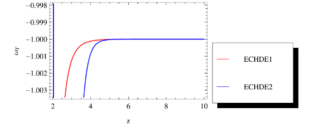
Figure 1. Plot of ωT versus z. The curves of the ECHDE model are characterized as follows: red is for the first category ( |
Considering the second category of scale factor (19 ), we can determine the density corresponding to the ECHDE model as $ \begin{eqnarray}{\rho }_{{\rm{\Lambda }}}=\displaystyle \frac{{\left(-1+h\right)}^{2}T\left({\left(-1+h\right)}^{2}T\beta -\tfrac{18{c}^{2}{h}^{2}}{{\kappa }^{2}}+{\left(-1+h\right)}^{2}T\alpha \mathrm{log}\left[-\tfrac{6{h}^{2}}{{\left(-1+h\right)}^{2}T{\kappa }^{2}}\right]\right)}{36{h}^{4}}.\end{eqnarray}$ Using the above procedure, the algebraic function corresponding to ECHDE model yields $ \begin{eqnarray}\begin{array}{rcl}f(T) & = & \displaystyle \frac{T\left(-162{c}^{2}{\left(-1+h\right)}^{2}{h}^{2}+162{h}^{4}+{\left(-1+h\right)}^{4}T(2\alpha +3\beta ){\kappa }^{2}\right)}{162{h}^{4}}\\ & & +\displaystyle \frac{T\left(3{\left(-1+h\right)}^{4}T\alpha {\kappa }^{2}\mathrm{log}\left[-\tfrac{6{h}^{2}}{{\left(-1+h\right)}^{2}T{\kappa }^{2}}\right]\right)}{162{h}^{4}}\\ & & +\sqrt{T}\left(-\displaystyle \frac{{\rm{\Lambda }}}{\sqrt{{T}_{0}}}+\displaystyle \frac{{c}^{2}{\left(-1+h\right)}^{2}\sqrt{{T}_{0}}}{{h}^{2}}\right)\\ & & -\sqrt{T}\left(\displaystyle \frac{{\left(-1+h\right)}^{4}{\kappa }^{2}\left(2\alpha +3\beta +3\alpha \mathrm{log}\left[-\tfrac{6{h}^{2}}{{\left(-1+h\right)}^{2}{\kappa }^{2}{T}_{0}}\right]\right){T}_{0}^{3/2}}{162{h}^{4}}\right),\end{array}\end{eqnarray}$ where we have used the boundary conditions (28 ) to determine the integration constant. Now, we can easily determine for this second category of scale factor, the EoS parameter corresponding to the algebraic function according to ECHDE model f(T)-gravity model $ \begin{eqnarray}\begin{array}{rcl}{\omega }_{T} & = & -1-\left\{\displaystyle \frac{4\left(18{c}^{2}{h}^{2}+{\left(-1+h\right)}^{2}T(\alpha -2\beta ){\kappa }^{2}\right)}{T\left(-18{c}^{2}{h}^{2}+{\left(-1+h\right)}^{2}T\beta {\kappa }^{2}+{\left(-1+h\right)}^{2}T\alpha {\kappa }^{2}\mathrm{log}\left[-\tfrac{6{h}^{2}}{{\left(-1+h\right)}^{2}T{\kappa }^{2}}\right]\right)}\right.\\ & & -\left.\displaystyle \frac{8\left({\left(-1+h\right)}^{2}T\alpha {\kappa }^{2}\mathrm{log}\left[-\tfrac{6{h}^{2}}{{\left(-1+h\right)}^{2}T{\kappa }^{2}}\right]\right)\dot{H}}{T\left(-18{c}^{2}{h}^{2}+{\left(-1+h\right)}^{2}T\beta {\kappa }^{2}+{\left(-1+h\right)}^{2}T\alpha {\kappa }^{2}\mathrm{log}\left[-\tfrac{6{h}^{2}}{{\left(-1+h\right)}^{2}T{\kappa }^{2}}\right]\right)}\right\},\end{array}\end{eqnarray}$ which can be rewritten under a form similar to the relation (34 ) $ \begin{eqnarray}\begin{array}{rcl}{\omega }_{T} & = & -1+\displaystyle \frac{2}{3\,h}\left\{-\displaystyle \frac{\left(3{c}^{2}{h}^{2}-{\left(-1+h\right)}^{2}{H}^{2}(\alpha -2\beta ){\kappa }^{2}\right)}{\left(3{c}^{2}{h}^{2}+{\left(-1+h\right)}^{2}{H}^{2}\beta {\kappa }^{2}+{\left(-1+h\right)}^{2}{H}^{2}\alpha {\kappa }^{2}\mathrm{log}\left[\tfrac{{h}^{2}}{{\left(-1+h\right)}^{2}{H}^{2}{\kappa }^{2}}\right]\right)}\right.\\ & & \left.+\displaystyle \frac{\left(2{\left(-1+h\right)}^{2}{H}^{2}\alpha {\kappa }^{2}\mathrm{log}\left[\tfrac{{h}^{2}}{{\left(-1+h\right)}^{2}{H}^{2}{\kappa }^{2}}\right]\right)\dot{H}}{\left(3{c}^{2}{h}^{2}+{\left(-1+h\right)}^{2}{H}^{2}\beta {\kappa }^{2}+{\left(-1+h\right)}^{2}{H}^{2}\alpha {\kappa }^{2}\mathrm{log}\left[\tfrac{{h}^{2}}{{\left(-1+h\right)}^{2}{H}^{2}{\kappa }^{2}}\right]\right)}\right\}.\end{array}\end{eqnarray}$ As observed previously in the case of the first class of the scaling factor, we note a phase transition between ${\omega }_{T}\gt -1$ and ${\omega }_{T}\lt -1$ which can be observed in the figure 1.
5. f(T) reconstruction from NADE model
The ADE model suggested by Cai in [21–23], describe the state of the Universe. In order to explain the matter-dominated epoch, the new agegraphic dark energy ADE (NADE) model was proposed by Wei and Cai [24], while the time scale was chosen to be the conformal time instead of the age of the Universe. The energy density and the conformal time corresponding to this model are given respectively by $ \begin{eqnarray}{\rho }_{{\rm{\Lambda }}}=\displaystyle \frac{3{n}^{2}}{{k}^{2}{\eta }^{2}},\end{eqnarray}$ and $ \begin{eqnarray}\eta =\int \displaystyle \frac{{\rm{d}}t}{a}=\int \displaystyle \frac{{\rm{d}}a}{{{Ha}}^{2}}.\end{eqnarray}$ Considering the first category of scale factor (17 ), and making use of equation (18 ), the conformal time η yields $ \begin{eqnarray}\eta ={\int }_{t}^{{t}_{s}}\displaystyle \frac{{\rm{d}}t}{a}=\displaystyle \frac{{\left({t}_{s}-t\right)}^{h+1}}{{a}_{0}(h+1)}=\displaystyle \frac{{h}^{h+1}}{{a}_{0}(h+1)}{\left(\displaystyle \frac{-6}{T}\right)}^{\tfrac{h+1}{2}}.\end{eqnarray}$ We can determine the corresponding density by replacing equation (51 ) into equation (49 ) $ \begin{eqnarray}{\rho }_{{\rm{\Lambda }}}=-\displaystyle \frac{{2}^{-1-h}{3}^{-h}{h}^{-2(1+h)}{\left(1+h\right)}^{2}{n}^{2}{\left(-\tfrac{1}{T}\right)}^{-h}{{Ta}}_{0}^{2}}{{\kappa }^{2}},\end{eqnarray}$ which yields to the differential equation where the solution is given by $ \begin{eqnarray}f(T)=T+\sqrt{T}{C}_{1}-\displaystyle \frac{{6}^{-h}{h}^{-2(1+h)}{\left(1+h\right)}^{2}{n}^{2}{\left(-\tfrac{1}{T}\right)}^{-h}{{Ta}}_{0}^{2}}{1+2h}.\end{eqnarray}$ Using the boundary conditions (28 ), we can obtain the integration constant as $ \begin{eqnarray}{C}_{1}=\displaystyle \frac{-2{\rm{\Lambda }}+\tfrac{{6}^{-h}{h}^{-2(1+h)}{\left(1+h\right)}^{2}{n}^{2}{a}_{0}^{2}\left(-\tfrac{1}{{T}_{0}}\right){}^{-h}{T}_{0}}{1+2h}}{\sqrt{{T}_{0}}},\end{eqnarray}$ Thus, we can determine f(T)-gravity model according to the NADE model as $ \begin{eqnarray}\begin{array}{rc}f(T) & \,=\,T+\displaystyle \frac{{6}^{-h}{h}^{-2(1+h)}{\left(1+h\right)}^{2}{n}^{2}{\left(-\tfrac{1}{T}\right)}^{-h}\sqrt{T}{a}_{0}^{2}\left(-\sqrt{T}\left(-\tfrac{1}{{T}_{0}}\right){}^{h}+{\left(-\tfrac{1}{T}\right)}^{h}\sqrt{{T}_{0}}\right)\left(-\tfrac{1}{{T}_{0}}\right){}^{-h}}{1+2h}-\displaystyle \frac{2\,\sqrt{T}{\rm{\Lambda }}}{\sqrt{{T}_{0}}}.\end{array}\end{eqnarray}$ Now, we can easily determine for this first category of scale factor, the EoS corresponding to the algebraic function according to the NADE as $ \begin{eqnarray}{\omega }_{T}=-1+\displaystyle \frac{4(1+h)\dot{H}}{T}.\end{eqnarray}$
Substituting equation (53 ) into equation (14 ), we get EoS corresponding to the algebraic function according to the NADE as $ \begin{eqnarray}{\omega }_{T}=-1-\displaystyle \frac{2(h+1)}{3h},\,\,\,h\gt 0.\end{eqnarray}$ We can note that the EoS parameter satisfies ${\omega }_{T}\lt -1$ which indicates to a accelerating expanded quintessence-like Universe.
Considering the second category of scale factor (19 ) and using (20 ) we obtain $ \begin{eqnarray}\begin{array}{l}\eta ={\int }_{0}^{t}\frac{{\rm{d}}t}{a}=\frac{{t}^{1-h}}{{a}_{0}(1-h)}=\frac{{h}^{1-h}}{{a}_{0}(1-h)}{\left(\frac{-6}{T}\right)}^{\tfrac{1-h}{2}},\\ \,\frac{1}{2}\lt h\lt 1.\end{array}\end{eqnarray}$ In order to preserve a real finite conformal time, it is necessary to have the condition $\tfrac{1}{2}\lt h\lt 1$ . Replacing equation (51 ) into (49 ) one can get the density $ \begin{eqnarray}{\rho }_{{\rm{\Lambda }}}=-\displaystyle \frac{{2}^{-1+h}{3}^{h}{\left(-1+h\right)}^{2}{h}^{-2+2h}{n}^{2}{\left(-\tfrac{1}{T}\right)}^{h}{{Ta}}_{0}^{2}}{{\kappa }^{2}},\end{eqnarray}$ and the algebraic function as $ \begin{eqnarray}f(T)=T+\sqrt{T}{C}_{1}+\displaystyle \frac{{6}^{h}{\left(-1+h\right)}^{2}{h}^{-2+2h}{n}^{2}{\left(-\tfrac{1}{T}\right)}^{h}{{Ta}}_{0}^{2}}{-1+2h},\end{eqnarray}$ where C1 is integration constant. Using the boundary conditions (28 ), the constant and the algebraic function f(T) are determined as $ \begin{eqnarray}{C}_{1}=\displaystyle \frac{-2{\rm{\Lambda }}+\tfrac{{6}^{h}{\left(-1+h\right)}^{2}{h}^{-2+2h}{n}^{2}{a}_{0}^{2}\left(-\tfrac{1}{{T}_{0}}\right){}^{-1+h}}{-1+2h}}{\sqrt{{T}_{0}}},\end{eqnarray}$ $ \begin{eqnarray}\begin{array}{l}f(T)=T\\ +\,\displaystyle \frac{{6}^{h}{\left(-1+h\right)}^{2}{h}^{-2+2h}{n}^{2}\sqrt{T}{a}_{0}^{2}\left({\left(-\tfrac{1}{T}\right)}^{h}\sqrt{T}-\left(-\tfrac{1}{{T}_{0}}\right){}^{h}\sqrt{{T}_{0}}\right)}{-1+2h}\\ -\,\displaystyle \frac{2\sqrt{T}{\rm{\Lambda }}}{\sqrt{{T}_{0}}}.\end{array}\end{eqnarray}$ Thus, we can deduce the EoS parameter as $ \begin{eqnarray}{\omega }_{T}=-1-\displaystyle \frac{4(-1+h)\dot{H}}{T},\end{eqnarray}$ which can be rewritten using (20 ) $ \begin{eqnarray}{\omega }_{T}=-1+\displaystyle \frac{2(1-h)}{3h},\,\,\,\displaystyle \frac{1}{2}\lt h\lt 1.\end{eqnarray}$ We can note that the EoS parameter satisfies $-1\lt {\omega }_{T}\lt -1/3$ which indicates to a accelerating expanded quintessence-like Universe.
6. f(T) reconstruction from ECNADE model
Based on a similar method to the ECHDE model, the ECNADE was suggested by Wei [20] and later by Karami [30] where the energy density is defined by $ \begin{eqnarray}{\rho }_{{\rm{\Lambda }}}=\displaystyle \frac{\alpha }{{\eta }^{4}}\mathrm{ln}\left(\displaystyle \frac{{\eta }^{2}}{{k}^{2}}\right)+\displaystyle \frac{\beta }{{\eta }^{4}}+\displaystyle \frac{3{n}^{2}}{{k}^{2}{\eta }^{2}}.\end{eqnarray}$
Considering the first category of scale factor (17 ) and replacing equation (51 ) into equation (65 ), the density corresponding becomes $ \begin{eqnarray}\begin{array}{l}{\rho }_{{\rm{\Lambda }}}=\displaystyle \frac{1}{{\kappa }^{2}}{36}^{-1-h}{h}^{-4(1+h)}{\left(1+h\right)}^{2}{\left(-\displaystyle \frac{1}{T}\right)}^{-2h}{{Ta}}_{0}^{2}\\ \times \,\left\{-{2}^{1+h}{3}^{2+h}{c}^{2}{h}^{2+2h}{\left(-\displaystyle \frac{1}{T}\right)}^{h}\right.\\ \left.+\,{\left(1+h\right)}^{2}T{\kappa }^{2}\left(\beta +\alpha \mathrm{log}\left[\displaystyle \frac{{6}^{1+h}{h}^{2+2h}{\left(-\tfrac{1}{T}\right)}^{1+h}}{{\left(1+h\right)}^{2}{\kappa }^{2}{a}_{0}^{2}}\right]\right){a}_{0}^{2}\right\}.\end{array}\end{eqnarray}$ Thus, the ECNADE f(T)-gravity model yields $ \begin{eqnarray}\begin{array}{rcl}f(T) & = & T+\sqrt{T}{C}_{1}-\displaystyle \frac{{6}^{-h}{c}^{2}{h}^{-2(1+h)}{\left(1+h\right)}^{2}{\left(-\tfrac{1}{T}\right)}^{-h}{{Ta}}_{0}^{2}}{1+2h}\\ & & +\displaystyle \frac{{2}^{-1-2h}{9}^{-1-h}{h}^{-4(1+h)}{\left(1+h\right)}^{4}{\left(-\tfrac{1}{T}\right)}^{-2h}{T}^{2}{\kappa }^{2}\left\{2(1+h)\alpha +(3+4h)\beta \right.}{{\left(3+4h\right)}^{2}}\\ & & +\displaystyle \frac{\left.(3+4h)\alpha \mathrm{log}\left[\tfrac{{6}^{1+h}{h}^{2+2h}{\left(-\tfrac{1}{T}\right)}^{1+h}}{{\left(1+h\right)}^{2}{\kappa }^{2}{a}_{0}^{2}}\right]\right\}{a}_{0}^{4}}{{\left(3+4h\right)}^{2}},\,\,\end{array}\end{eqnarray}$ where C1 is integration constant which can be determined from the boundary conditions (28 ) as $ \begin{eqnarray}\begin{array}{rcl}{C}_{1} & = & -\displaystyle \frac{{\rm{\Lambda }}}{\sqrt{{T}_{0}}}-\displaystyle \frac{{2}^{-1-2h}{9}^{-1-h}{h}^{-4(1+h)}{\left(1+h\right)}^{4}{\kappa }^{2}\left\{2(1+h)\alpha \right.}{\sqrt{{T}_{0}}{\left(3+4h\right)}^{2}}\\ & & +\displaystyle \frac{\left.(3+4h)\beta +(3+4h)\alpha \mathrm{log}\left[\tfrac{{6}^{1+h}{h}^{2+2h}\left(-\tfrac{1}{{T}_{0}}\right){}^{1+h}}{{\left(1+h\right)}^{2}{\kappa }^{2}{a}_{0}^{2}}\right]\right\}{a}_{0}^{4}\left(-\tfrac{1}{{T}_{0}}\right){}^{-2(1+h)}}{\sqrt{{T}_{0}}{\left(3+4h\right)}^{2}}\\ & & +\displaystyle \frac{{6}^{-h}{c}^{2}{h}^{-2(1+h)}{\left(1+h\right)}^{2}{a}_{0}^{2}\left(-\tfrac{1}{{T}_{0}}\right){}^{-h}{T}_{0}}{\sqrt{{T}_{0}}(1+2h)}.\end{array}\end{eqnarray}$ Therefore, the algebraic entropy-corrected ADE f(T)-gravity model reads $ \begin{eqnarray}\begin{array}{l}f(T)=T\\ +\,\displaystyle \frac{{6}^{-h}{c}^{2}{h}^{-2(1+h)}{\left(1+h\right)}^{2}{\left(-\tfrac{1}{T}\right)}^{-h}\sqrt{T}{a}_{0}^{2}\left\{-\sqrt{T}\left(-\tfrac{1}{{T}_{0}}\right){}^{h}\right.}{1+2h}\\ +\,\displaystyle \frac{\left.{\left(-\tfrac{1}{T}\right)}^{h}\sqrt{{T}_{0}}\right\}\left(-\tfrac{1}{{T}_{0}}\right){}^{-h}}{1+2h}-\displaystyle \frac{\sqrt{T}{\rm{\Lambda }}}{\sqrt{{T}_{0}}}\\ +\,\left\{\displaystyle \frac{1}{{\left(3+4h\right)}^{2}}{2}^{-1-2h}{9}^{-1-h}{h}^{-4(1+h)}{\left(1+h\right)}^{4}\right\}\\ \times \,\left\{{\left(-\displaystyle \frac{1}{T}\right)}^{-2h}\sqrt{T}{\kappa }^{2}{a}_{0}^{4}{\left(-\displaystyle \frac{1}{{T}_{0}}\right)}^{-2h}\right\}\\ \times \,\left\{({T}^{3/2}\left(2(1+h)\alpha +(3+4h)\beta +(3+4h)\alpha \right.\right.\\ \left.\times \,\mathrm{log}\left[\displaystyle \frac{{6}^{1+h}{h}^{2+2h}{\left(-\tfrac{1}{T}\right)}^{1+h}}{{\left(1+h\right)}^{2}{\kappa }^{2}{a}_{0}^{2}}\right]\right)\left(-\displaystyle \frac{1}{{T}_{0}}\right){}^{2h}\\ -\,{\left(-\displaystyle \frac{1}{T}\right)}^{2h}\left\{2(1+h)\alpha +(3+4h)\beta \right.\\ \left.\left.+\,(3+4h)\alpha \mathrm{log}\left[\displaystyle \frac{{6}^{1+h}{h}^{2+2h}\left(-\tfrac{1}{{T}_{0}}\right){}^{1+h}}{{\left(1+h\right)}^{2}{\kappa }^{2}{a}_{0}^{2}}\right]\right\}{T}_{0}^{3/2}\right\}.\end{array}\end{eqnarray}$ Substituting equation (72 ) into equation (14 ), the EoS parameter corresponding to algebraic function according to ECNADE model $ \begin{eqnarray}\begin{array}{rcl}{\omega }_{T} & = & -\left({2}^{1+h}{3}^{2+h}{c}^{2}{h}^{2+2h}{\left(-\displaystyle \frac{1}{T}\right)}^{h}\left(-T+4(1+h)\dot{H}\right)\right.\\ & & +\,{\left(1+h\right)}^{2}T{\kappa }^{2}{a}_{0}^{2}\left(T\left(\beta +\alpha \mathrm{log}\left[\displaystyle \frac{{6}^{1+h}{h}^{2+2h}{\left(-\tfrac{1}{T}\right)}^{1+h}}{{\left(1+h\right)}^{2}{\kappa }^{2}{a}_{0}^{2}}\right]\right)\right.\\ & & -\,\left.\left.4(1+h)\left(-\alpha +2\beta +2\alpha \mathrm{log}\left[\displaystyle \frac{{6}^{1+h}{h}^{2+2h}{\left(-\tfrac{1}{T}\right)}^{1+h}}{{\left(1+h\right)}^{2}{\kappa }^{2}{a}_{0}^{2}}\right]\right)\dot{H}\right)\right)\\ & & /\left(T\left(-{2}^{1+h}{3}^{2+h}{c}^{2}{h}^{2+2h}{\left(-\displaystyle \frac{1}{T}\right)}^{h}\right.\right.\\ & & +\,\left.\left.{\left(1+h\right)}^{2}T{\kappa }^{2}\left(\beta +\alpha \mathrm{log}\left[\displaystyle \frac{{6}^{1+h}{h}^{2+2h}{\left(-\tfrac{1}{T}\right)}^{1+h}}{{\left(1+h\right)}^{2}{\kappa }^{2}{a}_{0}^{2}}\right]\right){a}_{0}^{2}\right)\right).\end{array}\end{eqnarray}$
From the figure 2, we can remark that there is a phase transition between ${\omega }_{T}\gt -1$ and ${\omega }_{T}\lt -1$ .
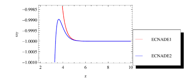
Figure 2. Plot of ωT versus z. The curves of the ECNADE model are characterized as follows: red is for the first category ( |
Considering the second category of scale factor (19 ), introducing equation (51 ) into equation (65 ) one obtains $ \begin{eqnarray}\begin{array}{rcl}{\rho }_{{\rm{\Lambda }}} & = & {6}^{-2+h}{\left(-1+h\right)}^{2}{h}^{-4+2h}{\left(-\displaystyle \frac{1}{T}\right)}^{h}\\ & & \times {{Ta}}_{0}^{2}\left\{-\displaystyle \frac{18{c}^{2}{h}^{2}}{{\kappa }^{2}}+{6}^{h}{\left(-1+h\right)}^{2}{h}^{2h}\right.\\ & & \left.\times {\left(-\displaystyle \frac{1}{T}\right)}^{h}T\left(\beta +\alpha \mathrm{log}\left[\displaystyle \frac{{6}^{1-h}{h}^{2-2h}{\left(-\tfrac{1}{T}\right)}^{1-h}}{{\left(-1+h\right)}^{2}{\kappa }^{2}{a}_{0}^{2}}\right]\right){a}_{0}^{2}\right\}.\end{array}\end{eqnarray}$ Solving the differential equation (11 ) for the energy density (66 ) yields $ \begin{eqnarray}\begin{array}{rcl}f(T) & = & T+\sqrt{T}{C}_{1}-\displaystyle \frac{{6}^{-h}{c}^{2}{h}^{-2(1+h)}{\left(1+h\right)}^{2}{\left(-\tfrac{1}{T}\right)}^{-h}{{Ta}}_{0}^{2}}{1+2h}\\ & & +\displaystyle \frac{{2}^{-1-2h}{9}^{-1-h}{h}^{-4(1+h)}{\left(1+h\right)}^{4}{\left(-\tfrac{1}{T}\right)}^{-2h}{T}^{2}{\kappa }^{2}{a}_{0}^{4}}{{\left(3+4h\right)}^{2}}\left\{2(1+h)\alpha +(3+4h)\beta \right.\\ & & \left.+(3+4h)\alpha \mathrm{log}\left[\displaystyle \frac{{6}^{1+h}{h}^{2+2h}{\left(-\tfrac{1}{T}\right)}^{1+h}}{{\left(1+h\right)}^{2}{\kappa }^{2}{a}_{0}^{2}}\right]\right\},\,\,\end{array}\end{eqnarray}$ where C1 is integration constant. Also C1 is determined from the boundary conditions (28 ) as $ \begin{eqnarray}\begin{array}{rcl}{C}_{1} & = & \displaystyle \frac{-{\rm{\Lambda }}-\tfrac{{2}^{-1-2h}{9}^{-1-h}{h}^{-4(1+h)}{\left(1+h\right)}^{4}{\kappa }^{2}\left\{2(1+h)\alpha +(3+4h)\beta +(3+4h)\alpha \mathrm{log}\left[\tfrac{{6}^{1+h}{h}^{2+2h}\left(-\tfrac{1}{{T}_{0}}\right){}^{1+h}}{{\left(1+h\right)}^{2}{\kappa }^{2}{a}_{0}^{2}}\right]\right\}{a}_{0}^{4}\left(-\tfrac{1}{{T}_{0}}\right){}^{-2(1+h)}}{{\left(3+4h\right)}^{2}}}{\sqrt{{T}_{0}}}\\ & & +\displaystyle \frac{\tfrac{{6}^{-h}{c}^{2}{h}^{-2(1+h)}{\left(1+h\right)}^{2}{a}_{0}^{2}\left(-\tfrac{1}{{T}_{0}}\right){}^{-h}{T}_{0}}{1+2h}}{\sqrt{{T}_{0}}}.\end{array}\end{eqnarray}$ Therefore, the algebraic function for the second class of scale factor (19 ) according to ECNADE model reads $ \begin{eqnarray}\begin{array}{rcl}f(T) & = & T+\displaystyle \frac{{6}^{-h}{c}^{2}{h}^{-2(1+h)}{\left(1+h\right)}^{2}{\left(-\tfrac{1}{T}\right)}^{-h}\sqrt{T}{a}_{0}^{2}\left(-\sqrt{T}\left(-\tfrac{1}{{T}_{0}}\right){}^{h}+{\left(-\tfrac{1}{T}\right)}^{h}\sqrt{{T}_{0}}\right)\left(-\tfrac{1}{{T}_{0}}\right){}^{-h}}{1+2h}-\displaystyle \frac{\sqrt{T}{\rm{\Lambda }}}{\sqrt{{T}_{0}}}\\ & & +\displaystyle \frac{1}{{\left(3+4h\right)}^{2}}{2}^{-1-2h}{9}^{-1-h}{h}^{-4(1+h)}{\left(1+h\right)}^{4}{\left(-\displaystyle \frac{1}{T}\right)}^{-2h}\sqrt{T}{\kappa }^{2}{a}_{0}^{4}\times \left(-\displaystyle \frac{1}{{T}_{0}}\right){}^{-2h}\\ & & \times \left\{{T}^{3/2}\left(2(1+h)\alpha +(3+4h)\beta \right.\right.\,\left.+(3+4h)\alpha \mathrm{log}\left[\displaystyle \frac{{6}^{1+h}{h}^{2+2h}{\left(-\tfrac{1}{T}\right)}^{1+h}}{{\left(1+h\right)}^{2}{\kappa }^{2}{a}_{0}^{2}}\right]\right)\\ & & \times \left(-\displaystyle \frac{1}{{T}_{0}}\right){}^{2h}-{\left(-\displaystyle \frac{1}{T}\right)}^{2h}\left(2(1+h)\alpha +(3+4h)\beta \right.\\ & & \left.\left.+(3+4h)\alpha \mathrm{log}\left[\displaystyle \frac{{6}^{1+h}{h}^{2+2h}\left(-\tfrac{1}{{T}_{0}}\right){}^{1+h}}{{\left(1+h\right)}^{2}{\kappa }^{2}{a}_{0}^{2}}\right]\right){T}_{0}^{3/2}\right\}.\end{array}\end{eqnarray}$ Introducing equation (72 ) into equation (14 ) yields the EoS parameter corresponding to the algebraic function according to the ECNADE model as $ \begin{eqnarray}\begin{array}{rcl}{\omega }_{T} & = & \left\{18{c}^{2}{h}^{2}\left(T+4(-1+h)\dot{H}\right)\right.-\,{6}^{h}{\left(-1+h\right)}^{2}{h}^{2h}{\left(-\displaystyle \frac{1}{T}\right)}^{h}T{\kappa }^{2}{a}_{0}^{2}\\ & & \times \,\left(T\left(\beta +\alpha \mathrm{log}\left[\displaystyle \frac{{6}^{1-h}{h}^{2-2h}{\left(-\tfrac{1}{T}\right)}^{1-h}}{{\left(-1+h\right)}^{2}{\kappa }^{2}{a}_{0}^{2}}\right]\right)\right.\\ & & +\,\left.\left.4(-1+h)\left(-\alpha +2\beta +2\alpha \mathrm{log}\left[\displaystyle \frac{{6}^{1-h}{h}^{2-2h}{\left(-\tfrac{1}{T}\right)}^{1-h}}{{\left(-1+h\right)}^{2}{\kappa }^{2}{a}_{0}^{2}}\right]\right)\dot{H}\right)\right\}\\ & & \div\,\left\{T\left(-18{c}^{2}{h}^{2}+{6}^{h}{\left(-1+h\right)}^{2}{h}^{2h}{\left(-\displaystyle \frac{1}{T}\right)}^{h}\right.\right.\\ & & \times \,\left.\left.T{\kappa }^{2}\left(\beta +\alpha \mathrm{log}\left[\displaystyle \frac{{6}^{1-h}{h}^{2-2h}{\left(-\tfrac{1}{T}\right)}^{1-h}}{{\left(-1+h\right)}^{2}{\kappa }^{2}{a}_{0}^{2}}\right]\right){a}_{0}^{2}\right)\right\}.\end{array}\end{eqnarray}$ From figure 2, we observe the same behavior.
7. Analysis of reconstructed model
In order to analyze the reconstructed models, we check in this section, the behavior of certain physical parameters as speed of sound and the Statefinder parameters. Squared speed of sound $ \begin{eqnarray}{v}_{s}^{2}=\displaystyle \frac{{\dot{p}}_{{\rm{eff}}}}{{\dot{\rho }}_{{\rm{eff}}}},\end{eqnarray}$ is an important quantity to test the stability of the background evolution. The study of the stability of the model will depend on the sign of equation (76 ). Several discussions were conducted leading to interesting results [28, 65–67]. We here considered the vs2 as equal to equation (76 ) and plot this vs2 verses the cosmic time z for both reconstructions of f(T) ECHDE and ECNADE models.
From the figure 3, we can observe the instability of ECHDE model for the two categories of scale factor 0 < z < 0.6 but the ECHDE model is stable when z > 0.6. The figure 4 indicates that the second category of scale factor corresponding to ECNADE model is unstable for 0 < z < 2 and stable when z > 2. On the other hand, for the first category corresponding to the ECNADE model remains stable for any value of z.
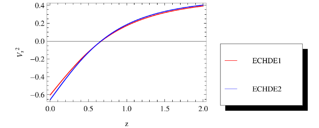
Figure 3. Plot of vs2 versus z. The curves of the ECHDE model are characterized as follows: red is for the first category ( |
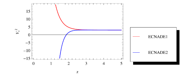
Figure 4. Plot of vs2 versus z. The curves of the ECNADE model are characterized as follows: red is for the first category ( |
8. Statefinder parameters
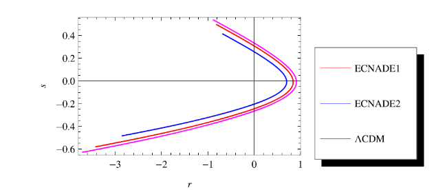
A series of candidates for the DE model have been suggested till date and some problems of competitivity are noted. In order to solve these problems, Sahni et al [68] introduced the statefinder $\{r,s\}$ diagnostic pair. This pair reads [68, 69] $ \begin{eqnarray}r=\displaystyle \frac{\dddot{a}}{{H}^{3}\,a},\quad s=\displaystyle \frac{r-1}{3\left(q-\tfrac{1}{2}\right)},\end{eqnarray}$ with q and H, respectively the deceleration and Hubble parameters. Thus, we can determine geometrically properties of DE. Interesting results have been found there [68–73]. We created the $\{r-s\}$ trajectories and compared with the ΛCDM limit based on the reconstructed models. We can observe from the figures 5 and 6 that although the trajectories approach the ΛCDM limit. Finally, the behavior of physical parameters as speed of sound and the Statefinder parameters is compatible with current observational data.
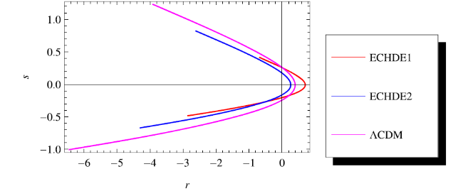
Figure 5. Plot of r versus s. The curves of the ECHDE model are characterized as follows: red is for the first category ( |
Figure 6. Plot of r versus s. The curves of the ECNADE model are characterized as follows: red is for the first category ( |
We see from figures 1 and 2 that the EoS parameter ωT is according to the current observational data. On the other hand, for the second class of scale factor, We can note from figures 1 and 2 that the EoS parameter satisfies $-1\lt {\omega }_{T}\lt -1/3$ which data indicates to a accelerating expanded quintessence-like Universe. By looking at the behavior of the curve shown in figure 2, in particular, the blue one, one can explicitly read that the effective EoS parameter can cross −1, which is also dubbed as the cosmological constant boundary. While it may be associated with some classical instability of cosmological perturbations, this phenomenon is often regarded as the quintom scenario, which has been discussed in [74]. In order to ensure the viability of the reconstructed models, we have performed a stability analysis by checking the behavior of certain physical parameters as speed of sound and the Statefinder parameters. From the figure 3, we can observe the instability of ECHDE model for the two class of scale factor 0 < z < 0.6 but the ECHDE model is stable when z > 0.6. The figure 4 indicates that the second category of scale factor from ECNADE model is unstable for 0 < z < 2 and stable when z > 2. On the other hand, for the first category of scale factor, the ECNADE model remains stable for any value of z. Finally, we have created the $\{r-s\}$ trajectories and compared with the ΛCDM limit. We can observe from the figures 5 and 6 that the trajectories approach the ΛCDM limit. Finally, the behavior of physical parameters as speed of sound and the Statefinder parameters are compatible with current observational data.
9. Conclusions
In this paper, we investigated how the theory of modified gravity f(T), where T denotes the torsion scalar, can describe the ECHDE and ECNADE models. To achieve our goal, we have reconstructed different algebraic functions according to the HDE, ECHDE, NADE and ECNADE models for the two classes of scale factor based on the f(T) action in the spatially flat FRW Universe (i) $a={a}_{0}{\left({t}_{s}-t\right)}^{-h}$ , (ii) $a={a}_{0}{t}^{h}$ . In addition, for the f(T) reconstructed models, we obtained the corresponding EoS parameters. The results show that for the first class of scale factor, the EoS parameter of the holographic and new agegraphic f(T)-gravity models always crosses the phantom-divide line, whereas for the second class, the EoS parameter of the mentioned models behaves like the quintessence EoS parameter. The EoS parameter of the entropy-corrected holographic and new agegraphic f(T)-gravity models for both classes of scale factors can accommodate the transition from quintessence state, ${\omega }_{T}\gt -1$ , to the phantom regime, ${\omega }_{T}\lt -1$ , as indicated by recent observations. For the third scale factor, the EoS parameter behaves like the cosmological constant. Also the f(T)-gravity models corresponding to the HDE, ECHDE, NADE and ECNADE can predict the early-time inflation of the Universe. In order to analyze the reconstructed models, we checked the behavior of certain physical parameters as speed of sound and the Statefinder parameters. We observed that the behavior of physical parameters approach the ΛCDM limit. Finally, the behavior of physical parameters as speed of sound and the Statefinder parameters are compatible with current observational data.