


1. Introduction
With the development of the national economy, traffic situations and traffic accidents are becoming increasingly serious. Traffic congestion has been a canonical problem in transportation science due to its complexity. To alleviate traffic congestion, extensive transportation management strategies have been proposed over the past decades, such as traffic accident analysis [1] and public transit operational strategies [1-3]. Traffic planners would benefit from a better understanding of driving behavior and an accurate estimation of traffic flow performance in order to effectively control the system. A distinct line of research concentrates on traffic flow modeling, to better understand the formation and propagation mechanism of traffic congestion.
Methodologically, traffic flow models can be divided into two categories: microscopic models and macroscopic models. The former group includes the cellular automaton models [4] and car-following models [5, 6], while the latter group includes the continuous models [7-9] and lattice models [10-16]. As opposed to the microscopic models, the macroscopic models are indifferent to the number of vehicles, such that less simulation and calculation time is required. This paper is concerned with the macroscopic models, more specifically the continuum models. The development of macro traffic flow models stems from the LWR model proposed by Lighthill, Whitham, and Richards [17], which was constructed based on the principle of conservation of vehicle flow. However, it was found that the LWR model is incapable of simulating non-equilibrium traffic phenomena such as stop-and-go traffic behaviors. To conquer this drawback, in 1971, Payne proposed a higher-order traffic model by replacing the equilibrium speed-density relationship with a dynamic equation for speed [18]. In 1995, Daganzo pointed out that the Payne model may violate the principle of anisotropy of traffic flow [19]. Later, Zhang [20] and Jiang et al [21] replaced the density gradient term in the Payne model with a velocity gradient term, such that the anisotropic characteristics of the traffic flow is satisfied, which paves the way for continuous flow modeling. Liu et al [22] proposed a continuum model considering the backward-looking effect, and they showed that the backward-looking effect can enhance the stability of traffic flow. Cheng et al [23], Zhai and Wu [24] added the traffic jerk term into the continuum model, which showed that traffic jams can be suppressed efficiently when the drivers can avoid an unnecessary jerk effect. Liu et al [25] and Cheng et al [26] investigated the impact of curved road and slopes in continuum models, and the results showed that the provision of friction and radius in curved roads can suppress traffic congestion, while the angle and slope length in road slopes also greatly affect the stability of traffic flow. Cheng et al [27] presented an extended continuum model accounting for the drivers' timid or aggressive attributes. Considering that electronic throttle (ET) angle information is one of the most important items of vehicle information in connected automatic vehicles, Li et al [28] and Jiao et al [29] introduced ET difference information into the continuous model. Other related studies can be found in the literature [8, 30-39].
In real traffic environments, car taillights are ubiquitous during the deceleration process. The driver of a following car can be informed of the car in front's status from the taillight. Intuitively, the driver of the following car tends to decelerate and keep a safe distance, given the preceding taillight. A recent study of a car-following model that considers the effect of a preceding taillight was done by Zhang et al [40]. They showed that the preceding vehicle's taillight information can greatly affect traffic flow stability. Later, Zhang et al [41] introduced the taillight effect into the macro traffic flow model. On the other hand, drivers often have a memory of historical information in the driving process. Although the effect of memory time has been investigated in the literature [42], the memory time of drivers is assumed to be a constant. Since the driving process is continuous, the above assumption is too strong. To be more realistic, we should consider the memory of drivers during a period of time [43, 44]. In summary, the aforementioned research was only done within the framework of micro traffic flow models, whereas macroscopic traffic flow models considering these realistic factors have been a rarity. Given the advantages of the macroscopic traffic flow models and their widespread application, there is an imminent need to develop a continuum model to address these concerns. As a remedy, this paper proposes a new continuum model with the driver's memory and the preceding vehicle's taillight. This research is expected to provide an insight into macroscopic traffic flow simulation and traffic control.
The reminder of this paper is as follows: a new continuous model considering the effect of the driver's memory time and the preceding vehicle's taillight is given in section 2 . The stability condition of the model is derived in section 3 . In section 4 , the KdV-Burgers equation is deduced through nonlinear analysis; the simulations carried out to verify the conclusions of the theoretical analysis are described in section 5 . Section 6 summarizes the main conclusions of this paper.
2. An extended continuum model
In 1995, Bando et al proposed an optimal velocity model (OVM) to describe car-following behavior in a single lane [45], specifically
$\begin{eqnarray}\displaystyle \frac{{\rm{d}}{v}_{n}(t)}{{\rm{d}}t}=a\left[V\left({\rm{\Delta }}{x}_{n}(t)\right)-{v}_{n}(t)\right],\end{eqnarray}$
where ${x}_{n}(t)$ and ${v}_{n}(t)$ are the instantaneous position and the velocity information of vehicle n at time t, respectively. ${\rm{\Delta }}{x}_{n}(t)$ is the headway between vehicle n and the vehicle (in front) n + 1 at time t, and ${\rm{\Delta }}{x}_{n}(t)={x}_{n+1}(t)-{x}_{n}(t).$ a is the driver's sensitivity. The optimal velocity function is a function of ${\rm{\Delta }}{x}_{n}(t),$ which takes the following form: $\begin{eqnarray}V\left({\rm{\Delta }}{x}_{n}(t)\right)=\displaystyle \frac{{v}_{\max }}{2}\left[\tanh \left({\rm{\Delta }}{x}_{n}(t)-{h}_{c}\right)+\,\tanh \left({h}_{c}\right)\right],\end{eqnarray}$
where ${h}_{c}$ is the safe distance, and ${v}_{\max }$ is the maximum velocity.The stability conditions can be obtained by carrying out a linear stability analysis of the above OVM, and the kink-antikink solitary wave solution obtained from the nonlinear stability analysis can be used to explain the propagation characteristics of traffic congestion. Given these advantages, many derivative models have been developed. Recently, a car-following model considering the drivers' memory times was proposed [46], which is expressed as follows:
$\begin{eqnarray}\displaystyle \frac{{\rm{d}}{v}_{n}(t)}{{\rm{d}}t}=a\left[V\left(\displaystyle \frac{1}{{\tau }_{0}}\displaystyle {\int }_{t-{\tau }_{0}}^{t}{\rm{\Delta }}{x}_{n}(u){\rm{d}}u\right)-{v}_{n}(t)\right]+\lambda {\rm{\Delta }}{v}_{n}(t),\end{eqnarray}$
where ${\tau }_{0}$ is the driver's sensory memory time, ${\rm{\Delta }}{v}_{n}(t)$ is the velocity difference between the vehicle n and the vehicle in front n + 1 at time t and $\lambda $ is the weighted parameter.In the absence of connected and automated vehicles, whether the current vehicle will adjust its speed is primarily dependent on the preceding vehicle's taillight. Intuitively, at the instant when the preceding vehicle's taillight comes on, the following vehicle tends to present braking behavior. In view of this, we introduce the preceding vehicle's taillight effect into equation (3 ); we then have an extended car-following model as follows:
$\begin{eqnarray}\displaystyle \frac{{\rm{d}}{v}_{n}(t)}{{\rm{d}}t}=a\left[V\left(\displaystyle \frac{1}{{\tau }_{0}}\displaystyle {\int }_{t-{\tau }_{0}}^{t}{\rm{\Delta }}{x}_{n}(u){\rm{d}}u\right)-{v}_{n}(t)\right]+\lambda {\rm{\Delta }}{v}_{n}(t)+{\theta }_{n}(t){\zeta }_{n}(t),\end{eqnarray}$
where ${\theta }_{n}(t)$ is a binary function indicating whether the front vehicle is decelerating, that is: $\begin{eqnarray}{\theta }_{n}(t)=\left\{\begin{array}{cc}0, & {a}_{n+1}\geqslant 0\\ 1, & {a}_{n+1}\lt 0\end{array}\right.,\end{eqnarray}$
where ${\zeta }_{n}(t)$ is a perturbation term induced by the preceding vehicle's taillight, which is defined as follows: $\begin{eqnarray}{\zeta }_{n}(t)=\left\{\begin{array}{ll}{\zeta }_{0}\,\tanh \left(1-\displaystyle \frac{h}{{x}_{0}}\right)\times H\left(-{\rm{\Delta }}{v}_{n}(t)\right)\times {\rm{\Delta }}{v}_{n}(t), & {\rm{\Delta }}\leqslant {x}_{0}\\ 0, & {\rm{\Delta }}\gt {x}_{0}\end{array}\right.,\end{eqnarray}$
where h is the headway between the following vehicle and the preceding vehicle. ${x}_{0}$ is the critical distance where the preceding vehicle's taillight takes effect on the following vehicle. ${\zeta }_{0}$ is a parameter that reflects the driver's characteristics. Generally, when $h\gt {x}_{0},$ the headway between adjacent vehicles is so large that the current vehicle is not affected by the preceding vehicle's taillight. On the contrary, when $h\leqslant {x}_{0},$ the distance between the two consecutive vehicles is close, such that the current vehicle should always pay attention to the preceding vehicle's taillight to avoid collisions. $H\left(\cdot \right)$ is the Heaviside function, specifically $\begin{eqnarray}H\left(x\right)=\left\{\begin{array}{ll}0, & x\geqslant 0\\ 1, & x\lt 0\end{array}\right..\end{eqnarray}$
In order to transform the above micro variables into macro variables, we transform the discrete variables of individual vehicles into continuous flow variables. We assume that the state of the vehicle n + 1 at position x represents the average traffic conditions in the region $\left[x-\tfrac{1}{2}h,x+\tfrac{1}{2}h\right],$ which is determined by the average traffic conditions in the preceding region $\left[x+\tfrac{1}{2}h,x+\tfrac{3}{2}h\right].$ Here, h corresponds to ${\rm{\Delta }}x$ in the car-following model and varies with the inter-vehicle space. As a result, the above micro variables can be transformed into macro variables, based on the method described in the literature [22]:
$\begin{eqnarray}\begin{array}{l}{v}_{n}(t)\to v(x,t),\,{v}_{n+1}(t)\to v(x+h,t),\\ V\left({\rm{\Delta }}{x}_{n}(t)\right)\to {V}_{e}\left(\rho \right),\,V^{\prime} \left({\rm{\Delta }}{x}_{n}(t)\right)\to \bar{V^{\prime} }\left(h\right),\\ V\left(\displaystyle \frac{1}{{\tau }_{0}}\displaystyle {\int }_{t-{\tau }_{0}}^{t}{\rm{\Delta }}{x}_{n}(u){\rm{d}}u\right)\to V\left(\displaystyle \frac{1}{{\tau }_{0}}\displaystyle {\int }_{t-{\tau }_{0}}^{t}h\left(x,t\right){\rm{d}}t\right),\end{array}\end{eqnarray}$
where $\rho (x,t)$ and $v(x,t)$ represent the macro density and the velocity at (x, t), respectively. h is the mean headway between two adjacent vehicles, and $h=\tfrac{1}{\rho }.$ ${V}_{e}\left(\rho \right)$ is the equilibrium speed, and$\bar{V^{\prime} }\left(h\right)=-{\rho }^{2}{V^{\prime} }_{e}\left(\rho \right).$Ignoring the higher-order nonlinear terms, we perform a Taylor expansion of $v(x+h,t),$ we then have
$\begin{eqnarray}v(x+h,t)=v(x,t)+h{v}_{x}+\displaystyle \frac{1}{2}{v}_{xx}{h}^{2}.\end{eqnarray}$
Substituting equations (8 ) and (9 ) into equation (4 ), we then have
$\begin{eqnarray}\begin{array}{l}\displaystyle \frac{\partial v}{\partial t}+\left[v-\left(\lambda +\phi \right)h\right]\displaystyle \frac{\partial v}{\partial x}=a\left[V\left(\displaystyle \frac{1}{{\tau }_{0}}\displaystyle {\int }_{t-{\tau }_{0}}^{t}h\left(x,t\right){\rm{d}}t\right)\right.\\ \,\,\,\,\,\,\,\,\,\,\,\,-\,\left.v(x,t)\Space{0ex}{3.0ex}{0ex}\right]+\displaystyle \frac{\left(\lambda +\phi \right)}{2}{v}_{xx}{h}^{2},\end{array}\end{eqnarray}$
where$\phi ={\zeta }_{0}\,\tanh \left(1-\tfrac{h}{{x}_{0}}\right).$Based on the intermediate value theorem, the following equation can then be obtained
$\begin{eqnarray}\begin{array}{l}V\left(\displaystyle \frac{1}{{\tau }_{0}}\displaystyle {\int }_{t-{\tau }_{0}}^{t}h\left(x,t\right){\rm{d}}t\right)={V}_{e}\left(\displaystyle \frac{1}{{\tau }_{0}}\displaystyle {\int }_{t-{\tau }_{0}}^{t}\rho \left(x,t\right){\rm{d}}ts\right)\\ \,\,\,\,\,\,\,\,=\,{V}_{e}\left(\rho \left(x,t-\mu {\tau }_{0}\right)\right),\end{array}\end{eqnarray}$
where $0\lt \mu \lt 1.$Performing a Taylor expansion of the items $\rho \left(x,t-\mu {\tau }_{0}\right)$ and ${V}_{e}\left(\rho \left(x,t-\mu {\tau }_{0}\right)\right),$ and ignoring the higher-order nonlinear terms, we then have
$\begin{eqnarray}\rho \left(x,t-\mu {\tau }_{0}\right)=\rho \left(x,t\right)-\mu {\tau }_{0}\displaystyle \frac{\partial \rho }{\partial t},\end{eqnarray}$
$\begin{eqnarray}{V}_{e}\left(\rho \left(x,t-\mu {\tau }_{0}\right)\right)={V}_{e}\left(\rho \left(x,t\right)\right)-\mu {\tau }_{0}{V^{\prime} }_{e}\left(\rho \right)\displaystyle \frac{\partial \rho }{\partial t}.\end{eqnarray}$
Combining equations (12 ) and (13 ) with the conservative equations yields a new continuum model with the driver's memory time and the preceding vehicle's taillight, as follows:
$\begin{eqnarray}\left\{\begin{array}{l}\displaystyle \frac{\partial \rho }{\partial t}+\rho \displaystyle \frac{\partial v}{\partial x}+v\displaystyle \frac{\partial \rho }{\partial x}=0\\ \displaystyle \frac{\partial v}{\partial t}+\left[v-\left(\lambda +\phi \right)h-a\mu {\tau }_{0}\rho {V^{\prime} }_{e}\left(\rho \right)\right]\displaystyle \frac{\partial v}{\partial x}=a\left[{V}_{e}\left(\rho \right)-v(x,t)\right]+a\mu {\tau }_{0}v{V^{\prime} }_{e}\left(\rho \right)\displaystyle \frac{\partial \rho }{\partial x}+\displaystyle \frac{\left(\lambda +\phi \right)}{2}{v}_{xx}{h}^{2}\end{array}\right..\end{eqnarray}$
3. Linear analysis
In this section, we perform a linear analysis on the extended continuum model. In order to facilitate subsequent derivation, equation (14 ) is rewritten as a vector form
$\begin{eqnarray}\displaystyle \frac{\partial U}{\partial t}+A\displaystyle \frac{\partial U}{\partial x}=E,\end{eqnarray}$
where $U=\left[\begin{array}{c}\rho \\ v\end{array}\right],$ $A=\left[\begin{array}{cc}v & \rho \\ -a\mu {\tau }_{0}v{V^{\prime} }_{e}\left(\rho \right) & v-\left(\lambda +\phi \right)h-a\mu {\tau }_{0}{V^{\prime} }_{e}\left(\rho \right)\rho \end{array}\right],$ $E=\left[\begin{array}{c}0\\ a\left[{V}_{e}\left(\rho \right)-v(x,t)\right]+\tfrac{\left(\lambda +\phi \right)}{2}{v}_{xx}{h}^{2}\end{array}\right].$Based on the roots obtained by solving the equation $\left|\lambda I-A\right|=0,$ the eigenvalues of A are
$\begin{eqnarray}\begin{array}{l}{\lambda }_{1}=v-\displaystyle \frac{\left(\lambda +\phi \right)h+a\mu {\tau }_{0}\rho {V^{\prime} }_{e}(\rho )+\sqrt{{\left[\left(\lambda +\phi \right)h+a\mu {\tau }_{0}\rho {V^{\prime} }_{e}(\rho )\right]}^{2}-4a\mu {\tau }_{0}{V^{\prime} }_{e}(\rho )v}}{2},\\ {\lambda }_{2}=v-\displaystyle \frac{\left(\lambda +\phi \right)h+a\mu {\tau }_{0}\rho {V^{\prime} }_{e}(\rho )-\sqrt{{\left[\left(\lambda +\phi \right)h+a\mu {\tau }_{0}\rho {V^{\prime} }_{e}(\rho )\right]}^{2}-4a\mu {\tau }_{0}{V^{\prime} }_{e}(\rho )v}}{2}.\end{array}\end{eqnarray}$
According to the above formula, there is no characteristic speed higher than the average speed v. This suggests that the new continuum model has an anisotropic property.
Subsequently, we conduct a qualitative analysis of the model based on the linear stability analysis method. To begin with, we assume that the initial traffic flow is uniform, and the steady-state solution for uniform flow is defined as
$\begin{eqnarray}\rho (x,t)={\rho }_{0},\,v(x,t)={v}_{0}.\end{eqnarray}$
A small perturbation is applied to the above uniform flow
$\begin{eqnarray}\left(\begin{array}{l}\rho (x,t)\\ v(x,t)\end{array}\right)=\left(\begin{array}{l}{\rho }_{0}\\ {v}_{0}\end{array}\right)+\left(\begin{array}{l}{\hat{\rho }}_{k}\\ {\hat{v}}_{k}\end{array}\right)\exp \left({\rm{i}}kx+{\sigma }_{k}t\right).\end{eqnarray}$
Substituting equation (18 ) into equation (14 ) and ignoring the higher-order nonlinear terms, we have that
$\begin{eqnarray}\left\{\begin{array}{l}\left({\sigma }_{k}+{v}_{0}{\rm{i}}k\right){\hat{\rho }}_{k}+{\rho }_{0}{\rm{i}}k{\hat{v}}_{k}=0\\ \left(-a{V^{\prime} }_{e}\left({\rho }_{0}\right)-a\mu {\tau }_{0}{v}_{0}{V^{\prime} }_{e}\left({\rho }_{0}\right){\rm{i}}k\right){\hat{\rho }}_{k}+\left\{\begin{array}{l}{\sigma }_{k}+\left[{v}_{0}-\left(\lambda +\phi \right)h-a\mu {\tau }_{0}{\rho }_{0}{V^{\prime} }_{e}\left({\rho }_{0}\right)\right]{\rm{i}}k+\\ a-\tfrac{\left(\lambda +\phi \right)}{2}{\left({\rm{i}}k\right)}^{2}{h}^{2}\end{array}\right\}{\hat{v}}_{k}=0\end{array}\right..\end{eqnarray}$
To ensure that the solution of equation (19 ) is non-zero, the necessary and sufficient condition is that the coefficient determinant is equal to zero, that is,
$\begin{eqnarray}\left|\begin{array}{cc}{\sigma }_{k}+{v}_{0}{\rm{i}}k & {\rho }_{0}{\rm{i}}k\\ -a{V^{\prime} }_{e}\left({\rho }_{0}\right)-a\mu {\tau }_{0}{v}_{0}{V^{\prime} }_{e}\left({\rho }_{0}\right){\rm{i}}k & \begin{array}{l}{\sigma }_{k}+\left[{v}_{0}-\left(\lambda +\phi \right)h-a\mu {\tau }_{0}{\rho }_{0}{V^{\prime} }_{e}\left({\rho }_{0}\right)\right]{\rm{i}}k+\\ a-\tfrac{\left(\lambda +\phi \right)}{2}{\left({\rm{i}}k\right)}^{2}{h}^{2}\end{array}\end{array}\right|=0.\end{eqnarray}$
After solving equation (20 ), we know that ${\sigma }_{k}$ satisfies the following conditions:
$\begin{eqnarray}\begin{array}{l}{\left({\sigma }_{k}+{v}_{0}{\rm{i}}k\right)}^{2}+\left({\sigma }_{k}+{v}_{0}{\rm{i}}k\right)\left\{\Space{0ex}{3.0ex}{0ex}a-\left[\left(\lambda +\phi \right)h\right.\right.\\ \,+\,\left.\left.a\mu {\tau }_{0}{\rho }_{0}{V^{\prime} }_{e}\left({\rho }_{0}\right)\right]{\rm{i}}k-\displaystyle \frac{\left(\lambda +\phi \right)}{2}{\left({\rm{i}}k\right)}^{2}{h}^{2}\right\}\\ \,+\,a{\rho }_{0}{V^{\prime} }_{e}\left({\rho }_{0}\right){\rm{i}}k\left(1+\mu {\tau }_{0}{v}_{0}{\rm{i}}k\right)=0.\end{array}\end{eqnarray}$
In order to determine the value of ${\sigma }_{k}$ in equation (21 ), we conduct a power series expansion of ${\sigma }_{k}$ by ik, that is,${\sigma }_{k}={\sigma }_{1}{\rm{i}}k+{\sigma }_{2}{\left({\rm{i}}k\right)}^{2}+\mathrm{...}.$ Substituting the above term into equation (21 ), we obtain the second-order expression of ik, which takes the following form:
$\begin{eqnarray}\begin{array}{l}\left[a\left({\sigma }_{1}+{v}_{0}\right)+a{\rho }_{0}{V^{\prime} }_{e}\left({\rho }_{0}\right)\right]{\rm{i}}k\\ \,+\,\left\{\begin{array}{l}{\left({\sigma }_{1}+{v}_{0}\right)}^{2}+a{\sigma }_{2}-\left({\sigma }_{1}+{v}_{0}\right)\left[\left(\lambda +\phi \right)h+a\mu {\tau }_{0}{\rho }_{0}{V^{\prime} }_{e}\left({\rho }_{0}\right)\right]\\ +a{\rho }_{0}{V^{\prime} }_{e}\left({\rho }_{0}\right)\mu {\tau }_{0}{v}_{0}\end{array}\right\}{\left({\rm{i}}k\right)}^{2}=0.\end{array}\end{eqnarray}$
To ensure the validity of the above equation, ik and the first- and second-order term coefficients in the formula should be equal to zero, from which the following equation can be obtained
$\begin{eqnarray}a\left({\sigma }_{1}+{v}_{0}\right)+a{\rho }_{0}{V^{\prime} }_{e}\left({\rho }_{0}\right)=0,\end{eqnarray}$
$\begin{eqnarray}\begin{array}{l}{\left({\sigma }_{1}+{v}_{0}\right)}^{2}+a{\sigma }_{2}-\left({\sigma }_{1}+{v}_{0}\right)\left[\left(\lambda +\phi \right)h+a\mu {\tau }_{0}{\rho }_{0}{V^{\prime} }_{e}\left({\rho }_{0}\right)\right]\\ \,+\,a{\rho }_{0}{V^{\prime} }_{e}\left({\rho }_{0}\right)\mu {\tau }_{0}{v}_{0}=0.\end{array}\end{eqnarray}$
Then the values of ${\sigma }_{1}$ and ${\sigma }_{2}$ are given
$\begin{eqnarray}\left\{\begin{array}{l}{\sigma }_{1}=-{v}_{0}-{\rho }_{0}{V^{\prime} }_{e}\left({\rho }_{0}\right)\\ {\sigma }_{2}=\displaystyle \frac{-{\left({\rho }_{0}{V^{\prime} }_{e}\left({\rho }_{0}\right)\right)}^{2}-{V^{\prime} }_{e}\left({\rho }_{0}\right)\left[\left(\lambda +\phi \right)h+a\mu {\tau }_{0}{\rho }_{0}{V^{\prime} }_{e}\left({\rho }_{0}\right)\right]}{a}-{\rho }_{0}{V^{\prime} }_{e}\left({\rho }_{0}\right)\mu {\tau }_{0}{v}_{0}\end{array}\right..\end{eqnarray}$
Based on the stability theory, the system is stable when ${\sigma }_{2}\gt 0.$ Hence, the neutral stability curve of the model is
$\begin{eqnarray}{a}_{s}=\displaystyle \frac{-{\rho }_{0}^{2}{V^{\prime} }_{e}\left({\rho }_{0}\right)-\left(\lambda +\phi \right)h}{{\rho }_{0}\mu {\tau }_{0}{v}_{0}+\mu {\tau }_{0}{\rho }_{0}{V^{\prime} }_{e}\left({\rho }_{0}\right)},\end{eqnarray}$
$\begin{eqnarray}\text{Im}\left({\sigma }_{k}\right)=-k\left[{v}_{0}+{\rho }_{0}{V^{\prime} }_{e}\left({\rho }_{0}\right)\right]+O\left({k}^{3}\right).\end{eqnarray}$
4. Nonlinear analysis
A new coordinate system is introduced into the new continuous traffic flow model, specifically:
$\begin{eqnarray}z=x-ct.\end{eqnarray}$
Substituting equation (28 ) into equation (14 ), equation (14 ) can be transformed into the following equation
$\begin{eqnarray}\left\{\begin{array}{l}-c{\rho }_{z}+{q}_{z}=0\\ -c{v}_{z}+\left[v-\left(\lambda +\phi \right)h-a\mu {\tau }_{0}\rho {V^{\prime} }_{e}\left(\rho \right)\right]{v}_{z}=a\left[{V}_{e}\left(\rho \right)-v\right]+a\mu {\tau }_{0}v{V^{\prime} }_{e}\left(\rho \right){\rho }_{z}+\displaystyle \frac{\left(\lambda +\phi \right)}{2}{v}_{zz}{h}^{2}\end{array}\right.,\end{eqnarray}$
where the flux is equal to the product of the density and the velocity, i.e., $q=\rho v.$From the first term of equation (29 ), we get
$\begin{eqnarray}{v}_{z}=\displaystyle \frac{c{\rho }_{z}}{\rho }-\displaystyle \frac{q{\rho }_{z}}{{\rho }^{2}}.\end{eqnarray}$
By the derivation of equation (30 ), we have that
$\begin{eqnarray}{v}_{zz}=\displaystyle \frac{c{\rho }_{zz}}{\rho }-\displaystyle \frac{2c{\rho }_{z}^{2}}{{\rho }^{2}}-\displaystyle \frac{q{\rho }_{zz}}{{\rho }^{2}}+\displaystyle \frac{2q{\rho }_{z}^{2}}{{\rho }^{3}}.\end{eqnarray}$
Based on the above analysis, the flow q can be expressed as
$\begin{eqnarray}q=\rho {V}_{e}(\rho )+{b}_{1}{\rho }_{z}+{b}_{2}{\rho }_{zz}.\end{eqnarray}$
Substituting equations (30 )-(32 ) into the second term of equation (29 ), equation (29 ) can then be transformed into
$\begin{eqnarray}\begin{array}{l}-c\left(\displaystyle \frac{c{\rho }_{z}}{\rho }-\displaystyle \frac{q{\rho }_{z}}{{\rho }^{2}}\right)+\left[\displaystyle \frac{q}{\rho }-\left(\lambda +\phi \right)h-a\mu {\tau }_{0}\rho {V^{\prime} }_{e}\left(\rho \right)\right]\\ \,\times \,\left(\displaystyle \frac{c{\rho }_{z}}{\rho }-\displaystyle \frac{q{\rho }_{z}}{{\rho }^{2}}\right)=a\left[{V}_{e}\left(\rho \right)-\displaystyle \frac{q}{\rho }\right]+a\mu {\tau }_{0}\displaystyle \frac{q}{\rho }{V^{\prime} }_{e}\left(\rho \right){\rho }_{z}\\ \,+\,\displaystyle \frac{\left(\lambda +\phi \right)}{2}{h}^{2}\left(\displaystyle \frac{c{\rho }_{zz}}{\rho }-\displaystyle \frac{2c{\rho }_{z}^{2}}{{\rho }^{2}}-\displaystyle \frac{q{\rho }_{zz}}{{\rho }^{2}}+\displaystyle \frac{2q{\rho }_{z}^{2}}{{\rho }^{3}}\right).\end{array}\end{eqnarray}$
Since ${\rho }_{z}$ and ${\rho }_{zz}$ are non-zero variables, the coefficients of ${\rho }_{z}$ and ${\rho }_{zz}$ in equation (33 ) equal zero. As a result, the following equations can be obtained
$\begin{eqnarray}\,\left\{\begin{array}{l}{b}_{1}=\mu {\tau }_{0}{V}_{e}(\rho ){V^{\prime} }_{e}\left(\rho \right)\rho +\displaystyle \frac{c\left(c-{V}_{e}(\rho )\right)-\left[{V}_{e}(\rho )-\left(\lambda +\phi \right)h-a\mu {\tau }_{0}\rho {V^{\prime} }_{e}\left(\rho \right)\right]\left(c-{V}_{e}(\rho )\right)}{a}\\ {b}_{2}=\displaystyle \frac{\left(\lambda +\phi \right)}{2a}{h}^{2}\left(c-{V}_{e}(\rho )\right)\end{array}\right..\end{eqnarray}$
Near the neutral stability curve, we set $\rho ={\rho }_{h}+\hat{\rho }(x,t).$ Expanding $\hat{\rho }$ to the second-order term, we have
$\begin{eqnarray}\begin{array}{l}\rho {V}_{e}(\rho )\approx {\rho }_{h}{V}_{e}({\rho }_{h})+{\left.{\left(\rho {V}_{e}(\rho )\right)}_{\rho }\right|}_{\rho ={\rho }_{h}}\hat{\rho }\\ \,\,\,\,+\,\displaystyle \frac{1}{2}{\left.{\left(\rho {V}_{e}(\rho )\right)}_{\rho \rho }\right|}_{\rho ={\rho }_{h}}{\hat{\rho }}^{2}.\end{array}\end{eqnarray}$
Substituting equations (32 ) and (35 ) into the first term of equation (29 ), we have
$\begin{eqnarray}-c{\rho }_{z}+\left[{\left(\rho {V}_{e}\right)}_{\rho }+{\left(\rho {V}_{e}\right)}_{\rho \rho }\rho \right]{\rho }_{z}+{b}_{1}{\rho }_{zz}+{b}_{2}{\rho }_{zzz}=0.\end{eqnarray}$
In order to convert equation (36 ) into the standard KdV-Burgers equation, we perform the following transformation
$\begin{eqnarray}U=-\left[{\left(\rho {V}_{e}\right)}_{\rho }+{\left(\rho {V}_{e}\right)}_{\rho \rho }\rho \right],X=mx,T=-mt.\end{eqnarray}$
Substituting equation (37 ) into equation (36 ) yields the following standard KdV-Burgers equation as follows
$\begin{eqnarray}{U}_{T}+U{U}_{X}+m{b}_{1}{U}_{XX}+{m}^{2}{b}_{2}{U}_{XXX}=0.\end{eqnarray}$
In equation (38 ), the corresponding solution is
$\begin{eqnarray}\,U=\displaystyle \frac{3{\left(-m{b}_{1}\right)}^{2}}{25\left(-{m}^{2}{b}_{2}\right)}\times \left[\begin{array}{l}1+2\,\tanh \left(\pm \displaystyle \frac{-m{b}_{1}}{10{m}^{2}}\right)\left(X+\displaystyle \frac{6{\left(-m{b}_{1}\right)}^{2}}{25\left(-{m}^{2}{b}_{2}\right)}T+{\zeta }_{0}\right)\\ +{\tanh }^{2}\left(\pm \displaystyle \frac{-m{b}_{1}}{10{m}^{2}}\right)\left(X+\displaystyle \frac{6{\left(-m{b}_{1}\right)}^{2}}{25\left(-{m}^{2}{b}_{2}\right)}T+{\zeta }_{0}\right)\end{array}\right],\end{eqnarray}$
where ${\zeta }_{0}$ is an arbitrary constant.5. Numerical simulations
5.1. Discretization and analysis
In this section, we will verify the conclusions of the above theoretical analysis by simulation. Before carrying out simulation, the new continuum model equation (14 ) needs to be discretized. To this end, we used the onward discrete model for the partial differential equations of equation (14 ), and then the discrete format of the continuous equation (14 ) is
$\begin{eqnarray}{\rho }_{i}^{j+1}={\rho }_{i}^{j}+\displaystyle \frac{{\rm{\Delta }}t}{{\rm{\Delta }}x}{\rho }_{i}^{j}\left({v}_{i}^{j}-{v}_{i+1}^{j}\right)+\displaystyle \frac{{\rm{\Delta }}t}{{\rm{\Delta }}x}{v}_{i}^{j}\left({\rho }_{i-1}^{j}-{\rho }_{i}^{j}\right),\end{eqnarray}$
(a) when ${v}_{i}^{j}\lt {c}_{i}^{j},$ the second equation in equation (14 ) takes the forward difference format, specifically
$\begin{eqnarray}\begin{array}{l}{v}_{i}^{j+1}={v}_{i}^{j}-\displaystyle \frac{{\rm{\Delta }}t}{{\rm{\Delta }}x}\left({v}_{i}^{j}-{c}_{i}^{j}\right)\left({v}_{i+1}^{j}-{v}_{i}^{j}\right)+a{\rm{\Delta }}t\left[{V}_{e}\left({\hat{\rho }}_{i}^{j}\right)-{v}_{i}^{j}\right]\\ \,\,\,+\,\displaystyle \frac{{\rm{\Delta }}t{c}_{i}^{j}}{2{\rho }_{i}^{j}{\left({\rm{\Delta }}x\right)}^{2}}\left({v}_{i+1}^{j}-2{v}_{i}^{j}+{v}_{i-1}^{j}\right),\end{array}\end{eqnarray}$
(b) when ${v}_{i}^{j}\geqslant {c}_{i}^{j},$ the second equation in equation (14 ) takes the backward difference format, specifically
$\begin{eqnarray}\begin{array}{l}{v}_{i}^{j+1}={v}_{i}^{j}-\displaystyle \frac{{\rm{\Delta }}t}{{\rm{\Delta }}x}\left({v}_{i}^{j}-{c}_{i}^{j}\right)\left({v}_{i}^{j}-{v}_{i-1}^{j}\right)+a{\rm{\Delta }}t\left[{V}_{e}\left({\hat{\rho }}_{i}^{j}\right)-{v}_{i}^{j}\right]\\ \,\,\,+\,\displaystyle \frac{{\rm{\Delta }}t{c}_{i}^{j}}{2{\rho }_{i}^{j}{\left({\rm{\Delta }}x\right)}^{2}}\left({v}_{i+1}^{j}-2{v}_{i}^{j}+{v}_{i-1}^{j}\right),\end{array}\end{eqnarray}$
where ${c}_{i}^{j}=\tfrac{\lambda +{\zeta }_{0}\,\tanh \left(1-\tfrac{1}{{\rho }_{i}^{j}{x}_{0}}\right)}{{\rho }_{i}^{j}},$ $\hat{\rho }(t)=\tfrac{{\tau }_{0}}{\displaystyle {\int }_{t-{\tau }_{0}}^{t}\tfrac{1}{\rho \left(x,t\right)}{\rm{d}}t}.$ ${\rho }_{i}^{j},$ ${v}_{i}^{j}$ are the density and velocity information of the conditions (i, j), respectively. ${\rm{\Delta }}t$ and ${\rm{\Delta }}x$ represent the time step and the space step, respectively.Herein, the average density function as proposed by Herrmann and Kerner [49] is adopted as the initial density, which is expressed as follows
$\begin{eqnarray}\begin{array}{l}\rho (x,0)={\rho }_{0}+{\rm{\Delta }}{\rho }_{0}\left\{{\cosh }^{-2}\left[\displaystyle \frac{160}{L}\left(x-\displaystyle \frac{5L}{16}\right)\right]\right.\\ \,\,\,\,-\,\left.\displaystyle \frac{1}{4}{\cosh }^{-2}\left[\displaystyle \frac{40}{L}\left(x-\displaystyle \frac{11L}{32}\right)\right]\right\},\end{array}\end{eqnarray}$
where the road length L = 32.2 km, and ${\rm{\Delta }}{\rho }_{0}$ is the density perturbation.To better reproduce the evolution of traffic congestion, the simulation environment is set as periodic boundary conditions. This enables better reproduction of the evolution of traffic congestion in a closed loop traffic environment. The initial density and velocity are set as follows:
$\begin{eqnarray}\rho \left(L,t\right)=\rho \left(0,t\right),\,v\left(L,t\right)=v\left(0,t\right).\end{eqnarray}$
Meanwhile, the equilibrium speed-density relationship proposed by Kerner and Konhauser [50] is introduced
$\begin{eqnarray}{V}_{e}(\rho )={v}_{f}\left[{\left(1+\exp \displaystyle \frac{\tfrac{\rho }{{\rho }_{m}}-0.25}{0.06}\right)}^{-1}-3.72\times {10}^{-6}\right],\end{eqnarray}$
where ${v}_{f}$ and ${\rho }_{m}$ are the free-flowing speed and the maximum allowable density along the road, respectively.The remaining default parameters are taken as follows:
$\begin{eqnarray}\begin{array}{l}{\rm{\Delta }}x=100\,m,\,{\rm{\Delta }}t=1\,s,a=0.2,\,{x}_{0}=100,\,{v}_{f}=30\,{\rm{m}}\,{{\rm{s}}}^{-1},\\ {\rho }_{m}=0.2\,{\rm{veh}}/{\rm{m}}{\rm{.}}\end{array}\end{eqnarray}$
Figure 1 shows the temporal and spatial evolution of the density waves for different initial densities ${\rho }_{0}.$ We found that the density waves are in a stable condition when ${\rho }_{0}=0.028\,{\rm{veh}}/{\rm{m}}.$ As the initial density ${\rho }_{0}$ increases from 0.028 veh/m to 0.068 veh/m, stop-and-go waves appear, as shown in figures 1(b) and (c). When the initial density ${\rho }_{0}$ exceeds 0.078 veh/m, the density waves return to the stable state. Hence, the stability of the traffic flow is greatly affected by the initial density. In this example, 0.078 veh/m (0.028 veh/m) is the upper (lower) bound of the density waves for the continuum model. The traffic jam will disappear when the density waves are outside the range between the upper bound and lower bounds. Taken together, the unstable region of the new continuum model is $0.028\,{\rm{veh}}/{\rm{m}}\lt {\rho }_{0}\,\lt 0.078\,{\rm{veh}}/{\rm{m}}.$
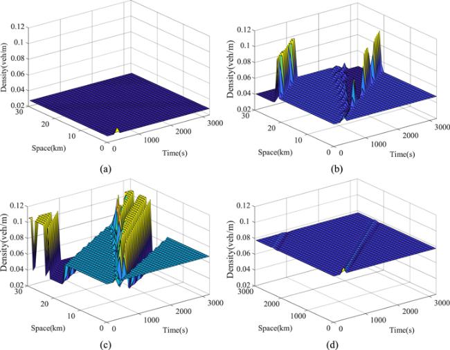
Figure 1. The spatiotemporal evolution of density waves with different values of the parameter ${\rho }_{0}:$ (a) ${\rho }_{0}=0.028{\rm{veh}}/{\rm{m}};$ (b) ${\rho }_{0}=0.048{\rm{veh}}/{\rm{m}};$ (c) ${\rho }_{0}=0.068{\rm{veh}}/{\rm{m}};$ (d) ${\rho }_{0}=0.078{\rm{veh}}/{\rm{m}}$ ($\lambda =0.6,$ ${\zeta }_{0}=0.3,$ ${\tau }_{0}=0.1$). |
Figure 2 presents the evolution of the density waves over time with different values of the parameter ${\tau }_{0},$ where figures 2(a)-(d) correspond to ${\tau }_{0}=0,0.1,0.2,0.3$ respectively. ${\tau }_{0}=0$ indicates that the driver is not affected by memory time during the driving process (figure 2(a)). Alternately, ${\tau }_{0}\gt 0$ indicates that the driver is constrained by memory time during the driving process (figures 2(b)-(d)). This shows that the fluctuating amplitude of the density waves becomes greater as the parameter ${\tau }_{0}$ increases, thereby aggravating the traffic jam. Figure 3 shows the instantaneous density distribution corresponding to figure 2 at t = 2000 s. One can see that the traffic density distribution is relatively smooth when ${\tau }_{0}=0$ compared with that when ${\tau }_{0}\gt 0.$ In other words, the traffic jam is less likely to take place in this condition, which is consistent with figure 2.
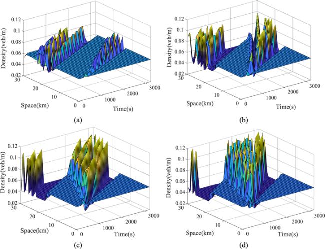
Figure 2. The spatiotemporal evolution of density waves under different values of parameter ${\tau }_{0}:$ (a) ${\tau }_{0}=0;$ (b) ${\tau }_{0}=0.1;$ (c) ${\tau }_{0}=0.2;$ (d) ${\tau }_{0}=0.3$ (${\rho }_{0}=0.06{\rm{veh}}/{\rm{m}},$ ${\zeta }_{0}=0.3,$ $\lambda =0.6$). |
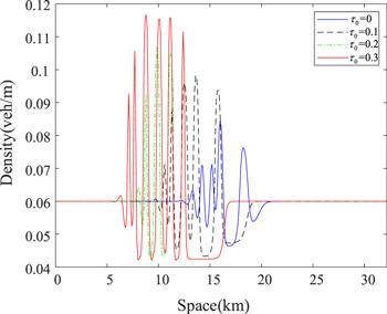
Figure 3. The density profiles at time t = 2000 corresponding to figure 2. |
Figures 4 and 5 analyze the relationship between the drivers' characteristic specific parameter ${\zeta }_{0}$ and traffic flow stability. We can see that the fluctuations in the amplitude of the density waves are large when ${\zeta }_{0}=0.25.$ With an increase of ${\zeta }_{0},$ the fluctuating amplitude and frequency are significantly decreased, and eventually reduced to zero when ${\zeta }_{0}=1.$ Therefore, a larger value of the parameter ${\zeta }_{0}$ contributes to mitigating traffic congestion and enhancing the model's robustness.
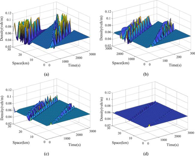
Figure 4. The spatiotemporal evolution of density waves under different values of the parameter ${\zeta }_{0}:$ (a) ${\zeta }_{0}=0.25;$ (b) ${\zeta }_{0}=0.5;$ (c) ${\zeta }_{0}=0.75;$ (d) ${\zeta }_{0}=1$ (${\rho }_{0}=0.06{\rm{veh}}/{\rm{m}},$ ${\tau }_{0}=0.1,$ $\lambda =0.7$) |
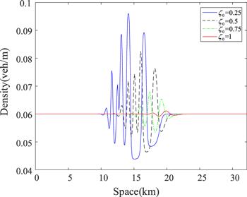
Figure 5. The density profiles at time t = 2000 s corresponding to figure 4. |
5.2. Energy consumption
Due to the limitations and potential pollution of fossil fuels, the energy consumption problem has raised many concerns in the traffic community. Traffic congestion is closely related to energy consumption. Generally, more congested traffic indicates a larger amount of energy consumption. In order to quantify the energy consumption, herein we adopt kinetic energy [29] to describe the amount of energy consumption, which takes the following form
$\begin{eqnarray}E\left(x,t\right)=\displaystyle \frac{1}{2}{v}^{2}(x,t).\end{eqnarray}$
The change of energy consumption on (x, t) is defined as follows:
$\begin{eqnarray}{\partial }_{t}E(x,t)=\displaystyle \frac{1}{2}{v}^{2}\left(x,t+{\rm{\Delta }}t\right)-\displaystyle \frac{1}{2}{v}^{2}\left(x,t\right),\end{eqnarray}$
$\begin{eqnarray}{\partial }_{x}E(x,t)=\displaystyle \frac{1}{2}{v}^{2}\left(x+{\rm{\Delta }}x,t\right)-\displaystyle \frac{1}{2}{v}^{2}\left(x,t\right).\end{eqnarray}$
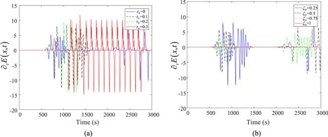
Figure 6 presents the distribution of the instantaneous energy consumption at different positions along the road for different values of the parameters ${\tau }_{0}$ and ${\zeta }_{0}$ at time t = 2000 s. Figure 7 shows the evolution of the energy consumption at the midpoint of the road during the time interval [zero s, 3000 s]. Figures 8 and 9 display the change patterns of energy consumption corresponding to figures 6 and 7. The change patterns of energy consumption in figures 8 and 9 are divided into two cases, namely ${\rm{\Delta }}E\gt 0$ and ${\rm{\Delta }}E\lt 0.$ When ${\rm{\Delta }}E\lt 0,$ vehicles are driving away from crowded roads, which corresponds to the release of energy consumption. Alternately, when ${\rm{\Delta }}E\gt 0,$ vehicles are decelerating into the congested road, which corresponds to the accumulation of energy consumption.

Figure 6. Instantaneous energy consumption distribution at different positions at t = 2000 s for different values of parameters (a) ${\tau }_{0}$ (${\zeta }_{0}=0.3,$ $\lambda =0.6,$ ${\rho }_{0}=0.06{\rm{veh}}/{\rm{m}}$); (b) ${\zeta }_{0}.$ (${\tau }_{0}=0.1,$ $\lambda =0.7,$ ${\rho }_{0}=0.06\,{\rm{veh}}/{\rm{m}}$). |
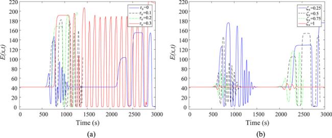
Figure 7. Evolution of the energy consumption at the midpoint of the road over time for different values of parameters (a) ${\tau }_{0}$ (${\zeta }_{0}=0.3,$ $\lambda =0.6,$ ${\rho }_{0}=0.06\,{\rm{veh}}/{\rm{m}}$); (b) ${\zeta }_{0}$ (${\tau }_{0}=0.1,$ $\lambda =0.7,$ ${\rho }_{0}=0.06\,{\rm{veh}}/{\rm{m}}$). |
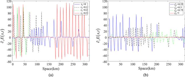
Figure 8. The change of energy consumption corresponding to figure 6. |
Figure 9. The change of energy consumption corresponding to figure 7. |
A list of findings can be summarized from figures 6-9: firstly, the parameter ${\tau }_{0}$ changes proportionally to the energy consumption, and the change of energy consumption is greater with the increase of parameter ${\tau }_{0}.$ Secondly, as for the parameter ${\zeta }_{0}$ the opposite conclusion applies. The energy consumption changes less as the parameter ${\zeta }_{0}$ increases, and it eventually returns to equilibrium when ${\zeta }_{0}=1.$ To sum up, the parameters ${\tau }_{0}$ and ${\zeta }_{0}$ have a significant impact on the energy consumed during the driving process.
6. Conclusion
In a real traffic environment, car taillights are not uncommon during the deceleration process, while drivers have a memory of historical information. The driving behavior and traffic flow performance are significantly complicated by these two factors. This paper develops a new continuum model with the driver's memory time and the preceding vehicle's taillight. The continuous driving process is also explicitly considered. We obtained the stability conditions and the KdV-Burgers equation for the new model. The solution can be used to explain the propagation and evolution mechanism of traffic density waves near the neutral stability curve. Through simulations we found that memory time and the preceding vehicle's taillight parameter contribute differently to the traffic jam. More specifically, increasing the memory time step ${\tau }_{0}$ hampers the stability of traffic flow, thereby aggravating traffic congestion and increasing energy consumption. On the contrary, a larger value of the parameter associated with the preceding vehicle's taillight ${\zeta }_{0}$ contributes to improving the model's robustness, thereby suppressing the traffic jam and reducing the energy consumption.
To the best of the authors' knowledge, this is the first paper on a continuum model with the driver's memory time and the preceding vehicle's taillight. This research is expected to provide insights for traffic simulation and software/platform development. Future research can incorporate the effects of driver heterogeneity and a fine-grained road environment. Furthermore, different types of vehicle may react differently to the vehicle's taillight. For example, trucks usually respond to the preceding vehicle's taillight more slowly, compared to private cars. Therefore, incorporating these realistic factors in the mixed traffic flow could be an interesting study. In addition, it would also be interesting to enhance the traffic flow module specifically in the simulation platform to guide traffic control practice.