


1. Introduction
Deep learning has garnered remarkable advances across diverse areas, including computer vision, speech recognition, language translation, natural language understanding, and other tasks [1], with the recent growth of big data and computing resources. It represents the data using multi-layer neural networks, i.e. deep neural networks. Despite the remarkable success in these and related areas, deep learning has not yet been widely used in the field of scientific computing. Moreover, its use in solving nonlinear evolution partial differential equations (PDEs) has emerged more recently [2-5].
PDEs have important applications in physics, engineering, biology, finance and other areas. Solving these equations has still been a computational challenge because many of these equations are difficult to be solved analytically or their analytical solution does not exist. Accordingly, solving them with neural networks as nonlinear approximators [6-10] is a very natural idea, and has been considered in several different forms previously [14-18]. The solution via deep learning method is closed analytic, differentiable and easy to be used in subsequent calculations compared with some traditional numerical approaches. In addition, the deep learning method does not require the discretization of spatial and temporal domains compared with other traditional numerical approaches.
Specifically, in this work, we solve nonlinear evolution equations by approximating the unknown solution with a deep neural network [26-28]. The network is trained to satisfy the equation and corresponding initial-boundary conditions. That is to say, with the help of the automatic differentiation techniques [11], the equation is embedded into the loss function in order to utilize the underlying laws of physics to discover patterns from experimental data. Moreover, this method requires much less data than ones proposed in other previous works [12].
Known that a specific setting that yields impressive results for certain equations could fail for some others, we just study second-order nonlinear evolution PDEs in one time and one space variable; that is, we consider the equations where each contains the dissipative term in addition to other partial derivatives. This family of equations has gained its importance because of applications across a range of scientific areas. Specifically, the equations that will be discussed in this paper, is of the form
$\begin{eqnarray}{u}_{t}-{u}_{{xx}}=P(u),\end{eqnarray}$
where the solution u is a function of the space variable x and the time variable t, and the term P(u) is a function of u and its derivatives. When $P(u)=-2{{uu}}_{x}$, we obtain the well-known Burgers' equation as the example in this paper. In addition, we will get the famous Fisher equation [13] when $P(u)\,=u(1-u)$.The paper is organized as follows. In section 2 , we introduce the neural network architecture and briefly present some problem setups. In section 3 , we consider a simple initial condition of the Burgers' equation to illustrate the algorithm. Then we give our main focus on the soliton phenomena of the Burgers' equation in section 4 . In section 5 , we demonstrate the capabilities of the algorithm for more general initial conditions of the Burgers' equation. Finally, we conclude the paper in section 6 .
2. Method
Although the existence of similar ideas for constraining neural network frameworks using some underlying physical laws (see, e.g. [14]), we revisit them using some more advanced tools, and then apply them to more challenging problems described by nonlinear evolution equations. Specifically, in this method, we approximate the solution u with a deep neural network and accordingly define a residual network to be given by
$\begin{eqnarray}f:= {u}_{t}-{ \mathcal N }(u,{u}_{x},{u}_{{xx}}),\end{eqnarray}$
where ${ \mathcal N }$ is a nonlinear function. The Burgers' equation corresponds to the case where ${ \mathcal N }={u}_{{xx}}-2{{uu}}_{x}$. Reference [26] also made more detailed analysis when including time t or space x, or both in ${ \mathcal N }$. By the way, ${ \mathcal N }$ can also be regarded as a nonlinear differential operator.We obtain the derivatives of the network u with respect to time t and space x using automatic differentiation with the aid of Tensorflow [19], which is a very popular and open-source deep learning software library.
Our main goal is to minimize the loss function3 ) attempts to fit the solution data and the second term learns to satisfy the residual f. Much research has been done on the convergence of the loss function (see, for example, [21]). In addition, whether there are other candidate objective functions or not will be the future research. In this paper, we just choose to optimize the loss function (3 ) using the L-BFGS algorithm. In addition, for larger datasets, more efficient algorithms can be readily employed, such as the stochastic gradient descent and Adam [20].
$\begin{eqnarray}L=\displaystyle \frac{1}{{N}_{u}}\displaystyle \sum _{i=1}^{{N}_{u}}| u({t}_{u}^{i},{x}_{u}^{i})-{u}^{i}{| }^{2}+\displaystyle \frac{1}{{N}_{f}}\displaystyle \sum _{j=1}^{{N}_{f}}| f({t}_{f}^{j},{x}_{f}^{j}){| }^{2},\end{eqnarray}$
where $\{{t}_{u}^{i},{x}_{u}^{i},{u}^{i}\}{}_{i=1}^{{N}_{u}}$ denote the initial-boundary training data on the solution network u and $\{{t}_{f}^{j},{x}_{f}^{j}\}{}_{j=1}^{{N}_{f}}$ specify the collocation points for the network f. The first term of the right hand side of equation (Throughout this work, we use relatively simple multi-layer perceptrons with the Xavier initialization and the hyperbolic tangent ($\tanh $) activation function. Commonly used initializations also include Gaussian initialization and He initialization; commonly used activations also include the sigmoid (σ) function and the rectified linear unit. In addition, we have tried some regularizations, such as batch normalization and dropout, it could not improve the expressiveness of the model and the performance sometimes becomes even worse. Therefore, we do not use additional regularizations except for the underlying laws expressed by the given equation in this paper. More detailed analysis will be conducted in future work.
In the following of this paper, we consider the (1+1)-dimensional Burgers' equation along with Dirichlet boundary conditions (other common boundary conditions also including Neumann boundary conditions and mixed boundary conditions):
$\begin{eqnarray}\left\{\begin{array}{l}{u}_{t}+2{{uu}}_{x}-{u}_{{xx}}=0,x\in [-20,20],t\in [-10,10],\\ u({t}_{0},x)={u}_{0}(x),\\ u(t,-20)=a,u(t,20)=b,\end{array}\right.\end{eqnarray}$
where ${u}_{0}(x)$ is certain initial function, and a, b are constants.Now, define $f(t,x)$ to be given by
$\begin{eqnarray}f:= {u}_{t}+2{{uu}}_{x}-{u}_{{xx}}.\end{eqnarray}$
To obtain the training and testing datasets, we simulate equation (4 ) using conventional spectral methods (for some kink-type soliton solutions, we just use certain PDE solvers in Matlab). Specifically, starting from an initial condition ${u}_{0}(x),x\in [-20,20]$ and assuming Dirichlet boundary conditions, we use the Chebfun package [22] with a Fourier discretization with 512 modes and a 4th-order explicit Runge-Kutta integrator with time-step size 1 × 10−04, and then integrate the equation up to the final time t = 10. The solution is saved every Δt = 0.1 to give us a total of 201 snapshots. Out of this dataset, we generate a smaller training subset by randomly subsampling Nu = 100 (usually relatively small) initial-boundary data and Nf = 10 000 collocation data points generated usually using the Latin hypercube sampling strategy [23].
In this work, we choose the neural network's architectures in a consistent fashion throughout the paper. Specifically, we represent the latent solution by a 13-layer deep neural network with 40 neurons per hidden layer. Furthermore, let ${ \mathcal N }$ be a specific physical prior, which is expressed by an equation rather than a neural network like with that of u [26]. We use $\tanh (x)$ as the activation function only in the hidden layers rather than the output layer. In addition, all experiments are conducted on a MacBook Pro computer with 2.4 GHz Dual-Core Intel Core i5 processor.
3. A simple example: trigonometric function
Let us start with a simple initial and boundary condition in order to highlight the ability of the method. Here, we consider a cosine initial condition and periodic boundary condition of equation (4 ) which are given by
$\begin{eqnarray}\left\{\begin{array}{l}{u}_{0}(x)=\cos \left(\tfrac{\pi (x+10)}{20}\right),\\ u(t,-20)=u(t,20)=0.\end{array}\right.\end{eqnarray}$
We know that the exact solution in this case is analytically available and relatively easy to solve. Figure 1 illustrates our result for the data-driven solution to the Burgers' equation. Specifically, given a set of initial and boundary data, we attempt to learn the latent solution u by training all learnable parameters of the network using the loss function (3 ). The top panel of figure 1 compares between the exact solution and the predicted spatiotemporal behavior. The resulting prediction error is measured at 9.21 × 10−03 in the relative ${{\mathbb{L}}}_{2}$-norm. Note that this prediction error is much lower than one reported in some previous works where they used other methods such as Gaussian processes [4]. A more detailed assessment of the predicted solution is presented in the bottom panel of figure 1. In particular, we present a comparison between the exact solution and predicted solution at different time points t = −7.5, −2.5, 7.5. Moreover, the algorithm can accurately capture the intrinsic and intricate nonlinear behavior of the Burgers' equation that leads to a shock around t = −2.0 using only a handful of data, while it is notoriously hard to accurately resolve with classical numerical methods and requires a laborious discretization of the equation [32].
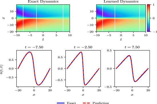
Figure 1. Cosine initial condition. Top: an exact solution to the Burgers' equation is compared to the corresponding solution of the learned PDE. The model correctly captures the dynamics behavior and accurately reproduces the solution with a relative ${{\mathbb{L}}}_{2}$ error of 9.21 × 10−03. Bottom: comparison between the predicted solutions and exact solutions at the three snapshots (corresponding to the vertical lines in the top panel). The model training took about 19 min. |
4. Soliton solutions
The soliton phenomena exist widespread in physics, biology, communications and other scientific disciplines. Although some exact and explicit soliton solutions of evolution equations can be obtained by the Darboux transformation, Hirota's direct method, and inverse scattering transform (see, e.g. [25]), these methods are relatively difficult to extend directly to other equations and there exist more unknown types of solitons. Specifically, we study the soliton behaviors of the Burgers' equation here.
4.1. One-soliton solution
First, we consider the one-soliton initial condition:
$\begin{eqnarray}{u}_{0}(x)=-\displaystyle \frac{k\exp \left(k(x-10k)\right)}{1+\exp \left(k(x-10k)\right)}.\end{eqnarray}$
Let k = 1, then we know that a = 0 and $b=-1$.
Figure 2 summarizes our results for one-soliton solution (the soliton is an anti-kink) to the Burgers' equation. The top panel of figure 2 compares between the exact solution and the predicted spatiotemporal behavior. The resulting prediction error is measured at 2.45 × 10−03 in the relative ${{\mathbb{L}}}_{2}$-norm. More detailed assessments of the predicted dynamics are presented in the middle and bottom panels, where the potential v = −ux is observed, of figure 2. In particular, we present a comparison between the exact solutions and predicted solutions at the three different time instants t = −7.5, −2.5, 7.5. The result indicates that the model can accurately capture the single soliton behavior of the Burgers' equation.
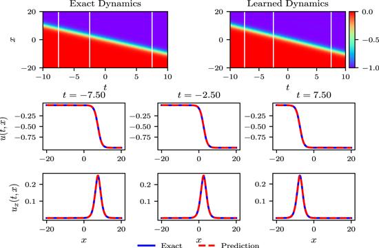
Figure 2. One-soliton solution. Top: an exact one-soliton solution to the Burgers' equation is compared to the solution of the learned PDE (right panel). The system correctly captures the dynamics and accurately reproduces the solution with a relative ${{\mathbb{L}}}_{2}$ error of 2.45 × 10−03. Middle: comparison of the predicted solutions and exact solutions at the three temporal snapshots. Bottom: comparison between the corresponding predicted and exact solutions of the potential. The training process took approximately half a minute. |
From figure 3, we can observe the single solitary wave motion better.
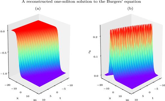
Figure 3. (a) The spatiotemporal behavior of the reconstructed single soliton. (b) The spatiotemporal dynamics of the corresponding potential. |
4.2. Two-soliton solutions
Then, we also consider the two-soliton initial condition:
$\begin{eqnarray}{u}_{0}(x)=-\displaystyle \frac{{k}_{1}\exp \left({k}_{1}(x-10{k}_{1})\right)+{k}_{2}\exp \left({k}_{2}(x-10{k}_{2})\right)}{1+\exp \left({k}_{1}(x-10{k}_{1})\right)+\exp \left({k}_{2}(x-10{k}_{2})\right)}.\end{eqnarray}$
When k1 = 1 and k2 = −1, we obtain a = 1, b = −1.
Figure 4 summarizes our results for the two-soliton solution to the Burgers' equation. The top panel of figure 4 compares between the exact dynamics and the predicted spatiotemporal behavior and the resulting prediction error is measured at 4.23 × 10−03 in the relative ${{\mathbb{L}}}_{2}$-norm. More detailed assessments of the predicted behavior are presented in the middle and bottom panels of figure 4. Moreover, we present a comparison between the exact solution and predicted solution at different time instants t = −7.5, −2.5, 7.5. The algorithm accurately recovers the two-soliton behavior of the Burgers' equation.
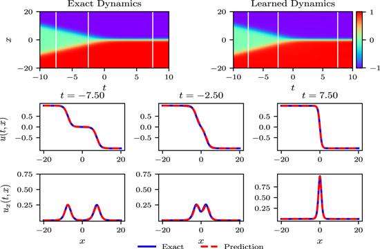
Figure 4. Two-soliton solution. Top: an exact two-soliton solution to the Burgers' equation (left panel) is compared to the corresponding reconstructed solution of the learned PDE. The system correctly captures the nonlinear dynamics and reproduces the solution with a relative ${{\mathbb{L}}}_{2}$ error of 4.23 × 10−03. Middle: comparison between the predicted and exact dynamics at the temporal snapshots. Bottom: comparison between the potential behaviors. The training took approximately 6.5 min. |
From figure 5, we can observe the soliton interaction better. In particular, we clearly see that the two solitons with same amplitudes fuse to one single soliton with a different amplitude at certain specific instant.
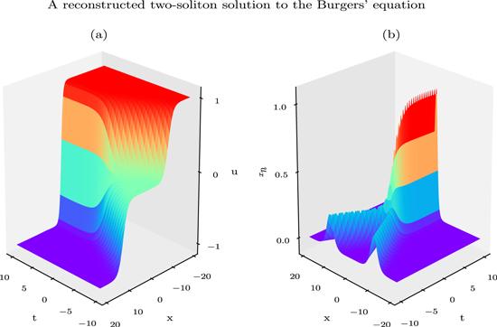
Figure 5. (a) The spatiotemporal behavior of the reconstructed two-soliton solution. (b) The nonlinear interaction of the corresponding potential. |
We consider another two-soliton solution when k1 = 1.5 and k2 = −1, which results in a = 1, b = −1.5.
Figure 6 summarizes our results for another two-soliton solution to the Burgers' equation. The top panel of figure 6 compares between the exact dynamics and the predicted spatiotemporal behavior. The prediction error is measured at 3.50 × 10−03 in the relative ${{\mathbb{L}}}_{2}$-norm. More detailed assessments of the predicted solution are presented in the middle and bottom panels of figure 6. In particular, we present a comparison between the exact solution and predicted solution at different instants t = −7.5, −2.5, 7.5. We find that the algorithm can also accurately capture the two-soliton behavior. From these experiments above, we just observe the soliton fusion behaviors of the Burgers' equation. More detailed analysis have been made, for example in [25]. In addition, the solution degenerates into a simple one-soliton solution whose wave dynamics is like that of section 4.1 when k1 = 1.5 and k2 = 1.0.
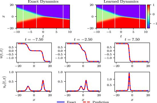
Figure 6. Another two-soliton solution. Top: an exact two-soliton solution to the Burgers' equation (left panel) is compared to the solution of the learned PDE. The system correctly captures the nonlinear dynamics and accurately reproduces the solution with a relative ${{\mathbb{L}}}_{2}$ error of 3.50 × 10−03. Middle: comparison between the predicted and exact solutions at the three temporal snapshots. Bottom: comparison between the corresponding predicted and exact solutions of the potential. The model training took about 3.5 min. |
From figure 7, we observe that the two single solitons with different amplitudes fuse into one soliton with an amplitude different from the first two again.
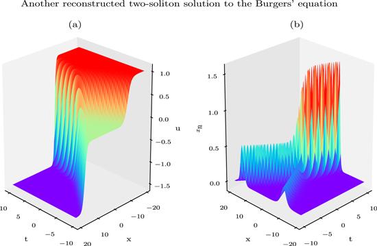
Figure 7. (a) The spatiotemporal behavior of another reconstructed two-soliton solution. (b) The nonlinear interaction of the corresponding potential. |
5. More complicated cases
More complicated and even unstable solutions rather than simple and stable solutions (e.g. solitons) often occur in the real world.
5.1. Exponential functions
First, we consider an exponential initial condition and periodic boundary condition of equation (4 ) given by
$\begin{eqnarray}\left\{\begin{array}{l}{u}_{0}(x)=-2\exp \left(-{\left(x+5\right)}^{2}\right),\\ u(t,-20)=u(t,20).\end{array}\right.\end{eqnarray}$
Figure 8 summarizes our results for the data-driven solution to the Burgers' equation. The top panel of figure 8 compares between the exact dynamics and the recovered behavior. The resulting prediction error is measured at 1.05 × 10−01 in the relative ${{\mathbb{L}}}_{2}$-norm, which is very large. A more detailed assessment of the predicted solution is presented in the bottom panel of figure 8. In particular, we present a comparison between the exact solution and the predicted solution at three different instants t = −7.5, −2.5, 7.5. From the bottom panel, we find that the algorithm can approximately capture the nonlinear behavior of the Burgers' equation. However, the dynamics is hard to accurately resolve from about t = −2.0, which remains unsolved in the current algorithm. It may require more finer-grained spatiotemporal data to be sampled [28], more network layers and hidden neurons [24, 29], even specific random seeds and more advanced network architectures [30-32]. We have made some preliminary experimental attempts, and more detailed analysis will be our future work.
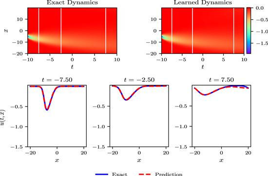
Figure 8. Exponential initial condition. Top: a solution to the Burgers' equation is compared to the corresponding solution to the learned PDE. The model approximately captures the nonlinear dynamics and reproduces the solution with a relative ${{\mathbb{L}}}_{2}$ error of 1.05 × 10−01. Bottom: comparison between the predicted solution and exact solution at the snapshots. The model training took approximately 12 min. |
Then, we consider another exponential initial condition and periodic boundary condition of equation (4 ) which are given by
$\begin{eqnarray}\left\{\begin{array}{l}{u}_{0}(x)=-2(x+5)\exp \left(-{\left(x+5\right)}^{2}\right),\\ u(t,-20)=u(t,20).\end{array}\right.\end{eqnarray}$
Unlike other cases considered in this paper, we just consider the nonlinear dynamics of the equation from t = −3.0 up to t = 3.0 here.
Figure 9 summarizes our results for the data-driven solution to the Burgers' equation. The top panel of figure 9 compares between the exact dynamics and the reconstructed spatiotemporal solution. Then the resulting error is measured at 1.97 × 10−02 in the relative ${{\mathbb{L}}}_{2}$-norm. A more detailed assessment of the predicted solution is presented in the bottom panel of figure 9. In particular, we present a comparison between the exact solution and the predicted solution at different moments t = −2.25, −0.75, 2.25. Compared to the previous case, the algorithm can accurately capture the complex nonlinear behavior of the Burgers' equation.
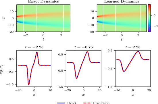
Figure 9. Another exponential initial condition. Top: a solution to the Burgers' equation is compared to the solution of the learned PDE. The system correctly captures the dynamics and reproduces the solution with a relative ${{\mathbb{L}}}_{2}$ error of 1.97 × 10−02. Bottom: comparison between the predicted and exact solutions at the three temporal snapshots. The training took about half an hour. |
5.2. Hyperbolic secant functions
In the following, we will study the hyperbolic secant (sech) function and related functions.
First, we consider a single sech initial condition and periodic boundary condition of equation (4 ) given by
$\begin{eqnarray}\left\{\begin{array}{l}{u}_{0}(x)=3{{\rm{sech}} }^{2}(x+5),\\ u(t,-20)=u(t,20).\end{array}\right.\end{eqnarray}$
Figure 10 summarizes our results for the data-driven solution to the Burgers' equation. The top panel of figure 10 compares between the exact dynamics and the predicted behavior and the resulting error is measured at 3.99 × 10−02 in the relative ${{\mathbb{L}}}_{2}$-norm. A more detailed assessment of the predicted behavior is presented in the bottom panel of figure 10. In particular, we present a comparison between the exact solution and the predicted solution at different instants t = −7.5, −2.5, 7.5. We see that the algorithm can accurately capture the nonlinear behavior of the Burgers' equation. Unlike the case (9 ), the model accurately resolve the nonlinear dynamics from about t = −2.0.
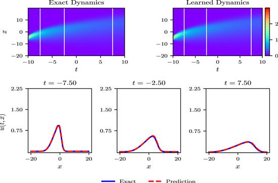
Figure 10. Hyperbolic secant initial condition. Top: a solution to the Burgers' equation is compared to the solution to the learned PDE. The system correctly captures the dynamics behavior and reproduces the solution with a relative ${{\mathbb{L}}}_{2}$ error of 3.99 × 10−02. Bottom: comparison between the predicted dynamics and the exact solution at the three temporal snapshots. The model training took approximately 7 min. |
Then, we consider a summation of two hyperbolic secant function and periodic boundary condition of equation (4 ) given by
$\begin{eqnarray}\left\{\begin{array}{l}{u}_{0}(x)=2{{\rm{sech}} }^{2}(x-2)+3{{\rm{sech}} }^{2}(x+5),\\ u(t,-20)=u(t,20).\end{array}\right.\end{eqnarray}$
Figure 11 summarizes our results for the data-driven solution to the Burgers' equation. The top panel of figure 11 compares between the exact dynamics and the predicted spatiotemporal solution. The prediction error is measured at 3.83 × 10−02 in the relative ${{\mathbb{L}}}_{2}$-norm. A more detailed assessment of the predicted solution is presented in the bottom panel of figure 11. In particular, we present a comparison between the exact dynamics and the predicted behavior at different time instants t = −7.5, −2.5, 7.5. The algorithm can accurately capture the nonlinear dynamics of the equation.
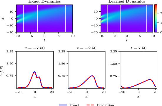
Figure 11. Second hyperbolic secant initial condition. Top: a solution to the Burgers' equation is compared to the solution of the learned PDE. The system correctly captures the dynamics and reproduces the solution with a relative ${{\mathbb{L}}}_{2}$ error of 3.83 × 10−02. Bottom: comparison between the predicted solution and the exact solution corresponding to the snapshots. The training took about 48 min. |
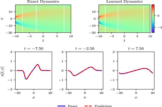
Furthermore, we also consider another initial condition and periodic boundary condition which are given by
$\begin{eqnarray}\left\{\begin{array}{l}{u}_{0}(x)=2{{\rm{sech}} }^{2}(x-2)-3{{\rm{sech}} }^{2}(x+5),\\ u(t,-20)=u(t,20).\end{array}\right.\end{eqnarray}$
Figure 12 summarizes our results for the data-driven solution to the Burgers' equation. The top panel of figure 12 compares between the exact dynamics and the predicted spatiotemporal dynamics and the resulting error is measured at 4.59 × 10−02 in the relative ${{\mathbb{L}}}_{2}$-norm. A more detailed assessment of the predicted dynamics is presented in the bottom panel of figure 12. In particular, we present a comparison between the exact solution and the predicted solution at different time instants t = −7.5, −2.5, 7.5. The algorithm can also accurately capture the nonlinear behavior of the Burgers' equation. In addition, it took much more time than the case (10 ).
Figure 12. Another hyperbolic secant initial condition. Top: a solution to the Burgers' equation is compared to the solution of the learned PDE. The system correctly captures the dynamics and reproduces the solution with a relative ${{\mathbb{L}}}_{2}$ error of 4.59 × 10−02. Bottom: comparison between the predicted solution and the exact solution at the snapshots. The training process took approximately 42 min. |
6. Remarks and discussion
In this paper, we present a neural network architecture for extracting nonlinear dynamics of PDEs from spatiotemporal data. The framework provides a universal treatment of (1+1)-dimensional second-order nonlinear evolution equations. The resulting method shows a pile of significant results for a diverse collection of initial-boundary conditions, including soliton solutions and other initial data. Relatively speaking, the more complex the initial data, the more time the model training takes. In particular, compared with other initial conditions, the training costs much less time for some soliton solutions perhaps because of the intrinsic structures of solitons.
Note that some of nonlinear evolution PDEs consist of terms like utt, uxt, $\sin (u)$ and some others. It would be very interesting to extend the network framework to incorporate such cases. It will be our future research.