


1. Introduction
Through the classical (local) nonlinear Schrödinger (NLS) equation $ \begin{eqnarray}{\rm{i}}{u}_{t}={u}_{{xx}}\pm 2| u{| }^{2}u,\end{eqnarray}$ the following nonlocal NLS equation $ \begin{eqnarray}{\rm{i}}{q}_{t}(x,t)={q}_{{xx}}(x,t)\pm 2q(x,t){q}^{* }(-x,t)q(x,t),\end{eqnarray}$ (where ∗ denotes complex conjugation and $q(x,t)$ is a complex valued function of the real variables x and t) or another elegant expression $ \begin{eqnarray}{\rm{}}\,{\rm{i}}{A}_{t}+{A}_{{xx}}\pm {A}^{2}B=0,B=\hat{f}A=\hat{P}\hat{C}A={A}^{* }(-x,t),\end{eqnarray}$ (where the operators $\hat{P}$ and $\hat{C}$ are the usual parity and charge conjugation) was introduced and investigated, which was called the parity-time reversal (PT) symmetric [1]. Except for the recent results, such as fractional optical solitons of the space-time fractional NLS equation [2], vector optical soliton and periodic solutions of a coupled fractional NLS equation [3], nonautonomous soliton solutions of variable-coefficient fractional NLS equation [4], the idea of the PT symmetry has wide applications in many areas of physics, such as the Bose–Einstein condensates [5], electric circuits [6], optics [7, 8], quantum chromodynamics [9], quantum physics [10].
Recent researches of the Alice–Bob (AB) systems were defined through the $\hat{P}\mbox{--}\hat{T}\mbox{--}\hat{C}$ (the parity, time reversal and charge conjugation) symmetry [11 –13]. Owing to this technical application, some typical integrable AB systems, such as the Korteweg–de Vries (KdV) [14, 15], the modified KdV [16 –19], the Boussinesq (Bq) [13], the Kadomtsev–Petviashvili (KP) [20, 21], the NLS [20, 21], the sine-Gordon [20] and the Toda lattice [11, 12] systems, were explicitly constructed and their invariant multiple soliton solutions were presented. Theoretically, the salient features of two correlated dipole blocking events in atmospheric dynamical systems were captured with the aid of the special approximate solutions [18, 19].
The well-known KP equation $ \begin{eqnarray}{u}_{{xt}}+3{\left({u}^{2}\right)}_{{xx}}+{u}_{{xxxx}}+3\kappa {u}_{{yy}}=0,\end{eqnarray}$ (with $\kappa =\pm 1$ ) is a universal model for the propagation of weakly nonlinear dispersive long waves, which are essentially one directional, with weak transverse effects [22]. Indeed, the extensions of the KP equation have been taken to deal with its physical restrictions, in which the constant coefficient ones attracted much more attention. In this paper, we focus our attention on the following KP equation $ \begin{eqnarray}{u}_{{xt}}+\alpha {\left({u}^{2}\right)}_{{xx}}+\beta {u}_{{xxxx}}+\sigma {u}_{{yy}}=0.\end{eqnarray}$ When the parameters $\alpha =6,\beta =1$ and σ be a nonnegative number, the KP equation (5 ) was studied as a natural extension of the classical KdV equation to two spatial dimensions, and was derived as a model for surface and internal water waves [23]. Its AB–KP system induced some invariant solutions including multiple soliton solutions, Painlevé reductions and soliton and p -wave interaction solutions [24]. Multisoliton solutions of this KP equation (5 ) describing nonlinear wave processes in media with positive dispersion were analyzed using exact and approximate methods [25]. Its conservation law was presented in the language of variational calculus and linear algebra through symbolic computation when $\beta =1$ [26]. Multi-component Wronskian solution [27], higher-order rational solitons and rogue-like wave solutions [28, 29] and obliquely propagating skew lumps [30] to the related KP equation were constructed, respectively. The complete integrability of the generalized variable-coefficient KP equation was investigated systematically under an integrable constraint condition [31, 32].
In the next several sections, we focus on the AB–KP system of the equation (5 ). In section 2 , a nonlocal AB–KP system is constructed and its bilinear formation is written through an extended Bäcklund transformation. In section 3 , the symmetry breaking soliton, symmetry breaking lump and symmetry breaking breather solutions according to the corresponding ansatze functions are presented through the derived Hirota bilinear formation of this AB–KP system. Some conclusions are given in the final section.
2. The AB–KP system and its bilinear formation
According to the principle of the AB system designed by Lou [11, 12], the AB–KP system is produced after substituting $u=\tfrac{1}{2}(A+B)$ into equation (5 ) $ \begin{eqnarray}\begin{array}{l}{A}_{{xt}}+{B}_{{xt}}+\displaystyle \frac{\alpha }{2}{[(A+B)({A}_{x}+{B}_{x})]}_{x}\\ \quad +\,\beta ({A}_{{xxxx}}+{B}_{{xxxx}})+\sigma ({A}_{{yy}}+{B}_{{yy}})=0,\end{array}\end{eqnarray}$ which can be split into the coupled system $ \begin{eqnarray}\begin{array}{l}{A}_{{xt}}+\displaystyle \frac{\alpha }{2}(A+B){A}_{{xx}}+\displaystyle \frac{\alpha }{4}{\left({A}_{x}+{B}_{x}\right)}^{2}\\ \quad +\,\beta {A}_{{xxxx}}+\sigma {A}_{{yy}}+{\rm{\Psi }}(A,B)=0,\end{array}\end{eqnarray}$ $ \begin{eqnarray}\begin{array}{l}{B}_{{xt}}+\displaystyle \frac{\alpha }{2}(A+B){B}_{{xx}}+\displaystyle \frac{\alpha }{4}{\left({A}_{x}+{B}_{x}\right)}^{2}\\ \quad +\,\beta {B}_{{xxxx}}+\sigma {B}_{{yy}}-{\rm{\Psi }}(A,B)=0,\end{array}\end{eqnarray}$ where B is related to A by $B={\hat{P}}_{s}^{x}{\hat{P}}_{s}^{y}{\hat{T}}_{d}A$ $=\,A(-x+{x}_{0},-y+{y}_{0},-t+{t}_{0})$ with arbitrary constants ${x}_{0},{y}_{0}$ and t 0 ( ${\hat{P}}_{s}^{x}{\hat{P}}_{s}^{y}{\hat{T}}_{d}$ expresses parities with shifts of the space variables x and y, time reversal with a delay). ${\rm{\Psi }}(A,B)$ is an arbitrary function of A and B, but should be ${\hat{P}}_{s}^{x}{\hat{P}}_{s}^{y}{\hat{T}}_{d}$ invariant. Although there are infinite functions satisfying this situation, system (7 ) can be simplified to the following AB–KP system when taking ${\rm{\Psi }}(A,B)=0$ $ \begin{eqnarray}{A}_{{xt}}=-\displaystyle \frac{\alpha }{2}(A+B){A}_{{xx}}-\displaystyle \frac{\alpha }{4}{\left({A}_{x}+{B}_{x}\right)}^{2}-\beta {A}_{{xxxx}}-\sigma {A}_{{yy}},\end{eqnarray}$ $ \begin{eqnarray}{B}_{{xt}}=-\displaystyle \frac{\alpha }{2}(A+B){B}_{{xx}}-\displaystyle \frac{\alpha }{4}{\left({A}_{x}+{B}_{x}\right)}^{2}-\beta {B}_{{xxxx}}-\sigma {B}_{{yy}}.\end{eqnarray}$
Now, we introduce an extended Bäcklund transformation $ \begin{eqnarray}\begin{array}{rcl}A & = & \displaystyle \frac{12\beta }{\alpha }{\left(\mathrm{ln}f\right)}_{{xx}}+a{\left(\mathrm{ln}f\right)}_{t}+b{\left(\mathrm{ln}f\right)}_{y}+c{\left(\mathrm{ln}f\right)}_{x},\\ B & = & \displaystyle \frac{12\beta }{\alpha }{\left(\mathrm{ln}f\right)}_{{xx}}-a{\left(\mathrm{ln}f\right)}_{t}-b{\left(\mathrm{ln}f\right)}_{y}-c{\left(\mathrm{ln}f\right)}_{x},\end{array}\end{eqnarray}$ with $a,b,c$ are three arbitrary constants and $f\equiv f(x,y,t)$ is an undetermined function of variables $x,y$ and t, which should also be ${\hat{P}}_{s}^{x}{\hat{P}}_{s}^{y}{\hat{T}}_{d}$ invariant, that is, $f(x,y,t)$ $=\,f(-x+{x}_{0},-y+{y}_{0},-t+{t}_{0})$ . If $a=b=c=0$ , equation (9 ) becomes a normal Bäcklund transformation. After substituting equation (9 ) into (8 ), the bilinear form of the AB–KP system can be expressed as $ \begin{eqnarray}({D}_{x}{D}_{t}+\beta {D}_{x}^{4}+\sigma {D}_{y}^{2})(f\cdot f)=0,\end{eqnarray}$ where ${D}_{x}{D}_{t},{D}_{x}^{4}$ and D y 2 are the bilinear derivative operators defined by [33, 34] $ \begin{eqnarray}\begin{array}{rcl}{D}_{x}^{m}{D}_{y}^{n}{D}_{t}^{l}(f\cdot g) & = & {\left(\displaystyle \frac{\partial }{\partial x}-\displaystyle \frac{\partial }{\partial x^{\prime} }\right)}^{m}{\left(\displaystyle \frac{\partial }{\partial y}-\displaystyle \frac{\partial }{\partial y^{\prime} }\right)}^{n}{\left(\displaystyle \frac{\partial }{\partial t}-\displaystyle \frac{\partial }{\partial t^{\prime} }\right)}^{l}\\ & & \times f(x,y,t)g(x^{\prime} ,y^{\prime} ,t^{\prime} ){| }_{x^{\prime} =x,y^{\prime} =y,t^{\prime} =t}.\end{array}\end{eqnarray}$
According to the properties of bilinear operator D, equation (10 ) is equal to $ \begin{eqnarray}{{ff}}_{{xt}}-{f}_{x}{f}_{t}+\beta ({{ff}}_{{xxxx}}-4{f}_{x}{f}_{{xxx}}+3{f}_{{xx}}^{2})+\sigma ({{ff}}_{{yy}}-{f}_{y}^{2})=0,\end{eqnarray}$ which is just a bilinear form of (8 ).
3. Symmetry breaking soliton, lump and breather solutions of the AB–KP system
In this section, we turn our attention to the Hirota bilinear formation (10 ) of the nonlocal AB–KP system (8 ) to derive the symmetry breaking soliton, symmetry breaking lump and symmetry breaking breather solutions, according to the corresponding ansatze functions.
| • | • Symmetry breaking soliton solution |
Based on the bilinear form (10 ) of the AB–KP system, the symmetry breaking multisoliton solution of equations (8 ) can be written as a summation of some special functions [11 –13, 24]. For example, we can choose $ \begin{eqnarray}\begin{array}{rcl}f & = & {f}_{n}=\displaystyle \sum _{\{\nu \}}{K}_{\{\nu \}}\cosh \left(\displaystyle \sum _{i=1}^{n}{\nu }_{i}{\xi }_{i}\right),\\ {\xi }_{i} & = & {k}_{i}\left[\left(x-\displaystyle \frac{{x}_{0}}{2}\right)+{l}_{i}\left(y-\displaystyle \frac{{y}_{0}}{2}\right)+{m}_{i}\left(t-\displaystyle \frac{{t}_{0}}{2}\right)\right],\\ {m}_{i} & = & -(4\beta {k}_{i}^{2}+\sigma {l}_{i}^{2}),\ \ {\nu }_{i}^{2}=1,\end{array}\end{eqnarray}$ where the summation of $\{\nu \}=\{{\nu }_{1},{\nu }_{2}$ , $\cdot \cdot \cdot ,{\nu }_{n}\}$ , and ${k}_{i},{l}_{j}(i,j=1,2,\cdot \cdot \cdot ,n)$ , ${x}_{0},{y}_{0},{t}_{0}$ are undetermined constants, while $ \begin{eqnarray}{K}_{\{\nu \}}=\displaystyle \prod _{i\lt j}^{n}{{\rm{\Delta }}}_{{ij}},\ \ {{\rm{\Delta }}}_{{ij}}^{2}=12{\left({k}_{i}+{\nu }_{i}{\nu }_{j}{k}_{j}\right)}^{2}\beta -{\left({l}_{i}-{l}_{j}\right)}^{2}\sigma .\end{eqnarray}$
3.1. Symmetry breaking line soliton solution
We take $ \begin{eqnarray}\begin{array}{rcl}f & = & {f}_{1}=\cosh ({\xi }_{1}),\\ {\xi }_{1} & = & {k}_{1}\left[\left(x-\displaystyle \frac{{x}_{0}}{2}\right)+{l}_{1}\left(y-\displaystyle \frac{{y}_{0}}{2}\right)+{m}_{1}\left(t-\displaystyle \frac{{t}_{0}}{2}\right)\right],\end{array}\end{eqnarray}$ with n = 1 of equation (13 ). By substituting equation (15 ) into (9 ), one can get the symmetry breaking line soliton solution of equations (8 ) $ \begin{eqnarray}{A}_{1}={k}_{1}({{am}}_{1}+{{bl}}_{1}+c)\tanh ({\xi }_{1})+\displaystyle \frac{12\beta {k}_{1}^{2}}{\alpha {\cosh }^{2}({\xi }_{1})},\end{eqnarray}$ $ \begin{eqnarray}{B}_{1}=-{k}_{1}({{am}}_{1}+{{bl}}_{1}+c)\tanh ({\xi }_{1})+\displaystyle \frac{12\beta {k}_{1}^{2}}{\alpha {\cosh }^{2}({\xi }_{1})},\end{eqnarray}$ with ${m}_{1}=-(4\beta {k}_{1}^{2}+\sigma {l}_{1}^{2})$ because of equation (10 ). As the existence of the hyperbolic function tanh term which makes ${B}_{1}={\hat{P}}_{s}^{x}{\hat{P}}_{s}^{y}{\hat{T}}_{d}{A}_{1}$ or ${A}_{1}={\hat{P}}_{s}^{x}{\hat{P}}_{s}^{y}{\hat{T}}_{d}{B}_{1}$ , the line soliton solution (16 ) of the AB–KP system (8 ) is ${\hat{P}}_{s}^{x}{\hat{P}}_{s}^{y}{\hat{T}}_{d}$ symmetric breaking solution.
Figures 1 (a) and (b) are two corresponding symmetric breaking line solitons when the constants are taken as $a=b=c=\beta ={k}_{1}={l}_{1}=1$ , ${x}_{0}={y}_{0}={t}_{0}=4$ , the others are $\alpha =\tfrac{12}{5},\sigma =-3,{m}_{1}=-1$ at time t = 0. Figures 1 (c) and (d) are the contour plots of these structures in the $(x,A/B)$ -plane, when taking the constant $c=0,2,4$ and 10, respectively. As the parameter c increases, the line soliton pairs trend to two symmetry breaking kinks.
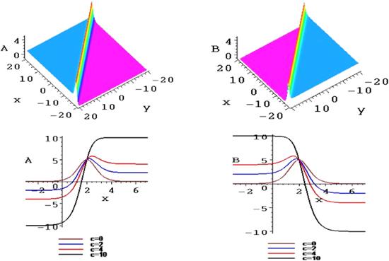
Figure 1. Plots of the symmetry breaking line solitons of A 1 and B 1 of the solution ( |
3.2. Interaction of the double symmetry breaking line solitons
According to equations (10 ), (13 ) and (14 ), the interaction solution of double symmetry breaking line solitons of equations (8 ) can be expressed as $ \begin{eqnarray}\begin{array}{rcl}{A}_{2} & = & \displaystyle \frac{12\beta }{\alpha }{\left(\mathrm{ln}{f}_{2}\right)}_{{xx}}+a{\left(\mathrm{ln}{f}_{2}\right)}_{t}+b{\left(\mathrm{ln}{f}_{2}\right)}_{y}+c{\left(\mathrm{ln}{f}_{2}\right)}_{x},\\ {B}_{2} & = & \displaystyle \frac{12\beta }{\alpha }{\left(\mathrm{ln}{f}_{2}\right)}_{{xx}}-a{\left(\mathrm{ln}{f}_{2}\right)}_{t}-b{\left(\mathrm{ln}{f}_{2}\right)}_{y}-c{\left(\mathrm{ln}{f}_{2}\right)}_{x},\end{array}\end{eqnarray}$ with $ \begin{eqnarray}\begin{array}{rcl}{f}_{2} & = & {\delta }_{+}\sqrt{12{\left({k}_{1}-{k}_{2}\right)}^{2}\beta -{\left({l}_{1}-{l}_{2}\right)}^{2}\sigma }\cosh ({\xi }_{1}+{\xi }_{2})\\ & & +{\delta }_{-}\sqrt{12{\left({k}_{1}+{k}_{2}\right)}^{2}\beta -{\left({l}_{1}-{l}_{2}\right)}^{2}\sigma }\cosh ({\xi }_{1}-{\xi }_{2}),\\ {\delta }_{+}^{2} & = & {\delta }_{-}^{2}=1,\end{array}\end{eqnarray}$ and $ \begin{eqnarray}\begin{array}{rcl}{\xi }_{i} & = & {k}_{i}\left[\left(x-\displaystyle \frac{{x}_{0}}{2}\right)+{l}_{i}\left(y-\displaystyle \frac{{y}_{0}}{2}\right)+{m}_{i}\left(t-\displaystyle \frac{{t}_{0}}{2}\right)\right],\\ {m}_{i} & = & -(4\beta {k}_{i}^{2}+\sigma {l}_{i}^{2}),\ \ i=1,2.\end{array}\end{eqnarray}$
We can verify that this is the ‘parities with shifts of the space variables x and y, time reversal with a delay’ invariant solution of equations (8 ). That is, ${B}_{2}={\hat{P}}_{s}^{x}{\hat{P}}_{s}^{y}{\hat{T}}_{d}{A}_{2}$ or ${A}_{2}\,={\hat{P}}_{s}^{x}{\hat{P}}_{s}^{y}{\hat{T}}_{d}{B}_{2}$ .
For example, when taking the constants $a=b=c\,=\beta ={k}_{1}={l}_{1}$ $=\,{\delta }_{+}={\delta }_{-}=1$ , ${x}_{0}={y}_{0}={t}_{0}=4$ , the others are $\alpha =\tfrac{12}{5},\sigma =-3$ , ${m}_{1}={k}_{2}=-1,{l}_{2}=-\tfrac{1}{2}$ , ${m}_{2}=-\tfrac{13}{4}$ , two corresponding interactions of the symmetry breaking line solitons are presented at time t = 0 (figure 2 ). Figures 3 and 4 are the contour plots of these structures in the $(x,A/B)$ -plane, taking $c=0,2,4$ and 10 at different times t = 0, 3 and 6, respectively. As the parameter c and the time t increase, the interactions of the symmetry breaking line soliton solution of equation (17 ) also trend to two symmetry breaking kinks.
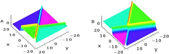
Figure 2. The interactions of the symmetry breaking line solitons of A 2 and B 2 of the solution ( |
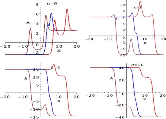
Figure 3. The contour plots of the interaction of the symmetry breaking line solitons A 2 with |
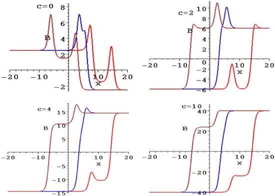
Figure 4. The contour plots of the interaction of the symmetry breaking line solitons B 2 with |
3.3. Interactions of the multifold symmetry breaking solitons
For n = 3, the solution (13 ) possesses the following form $ \begin{eqnarray}\begin{array}{rcl}f & \equiv & {f}_{3}={K}_{\{\}}\cosh ({\xi }_{1}+{\xi }_{2}+{\xi }_{3})\\ & & +{K}_{\{1\}}\cosh ({\xi }_{1}-{\xi }_{2}-{\xi }_{3})+{K}_{\{2\}}\cosh ({\xi }_{1}-{\xi }_{2}+{\xi }_{3})\\ & & +{K}_{\{3\}}\cosh ({\xi }_{1}+{\xi }_{2}-{\xi }_{3}),\end{array}\end{eqnarray}$ where $ \begin{eqnarray}\begin{array}{rcl}{K}_{\{\}} & = & {{\rm{\Delta }}}_{12}^{+}{{\rm{\Delta }}}_{13}^{+}{{\rm{\Delta }}}_{23}^{+},\ {K}_{\{1\}}={{\rm{\Delta }}}_{12}^{-}{{\rm{\Delta }}}_{13}^{-}{{\rm{\Delta }}}_{23}^{+},\\ {K}_{\{2\}} & = & {{\rm{\Delta }}}_{12}^{-}{{\rm{\Delta }}}_{13}^{+}{{\rm{\Delta }}}_{23}^{-},\ {K}_{\{3\}}={{\rm{\Delta }}}_{12}^{+}{{\rm{\Delta }}}_{13}^{-}{{\rm{\Delta }}}_{23}^{-},\end{array}\end{eqnarray}$ $ \begin{eqnarray}\begin{array}{rcl}{{\rm{\Delta }}}_{{ij}}^{\pm } & = & \sqrt{12{\left({k}_{i}\mp {k}_{j}\right)}^{2}\beta -{\left({l}_{i}-{l}_{j}\right)}^{2}\sigma },\\ {\xi }_{i} & = & {k}_{i}\left[\left(x-\displaystyle \frac{{x}_{0}}{2}\right)+{l}_{i}\left(y-\displaystyle \frac{{y}_{0}}{2}\right)+{m}_{i}\left(t-\displaystyle \frac{{t}_{0}}{2}\right)\right],\\ {m}_{i} & = & -(4\beta {k}_{i}^{2}+\sigma {l}_{i}^{2}),\ \ (i,j=1,2,3).\end{array}\end{eqnarray}$ Therefore, the interaction solution of the triple symmetry breaking solitons of equations (8 ) can be expressed as $ \begin{eqnarray}\begin{array}{rcl}{A}_{3} & = & \displaystyle \frac{12\beta }{\alpha }{\left(\mathrm{ln}{f}_{3}\right)}_{{xx}}+a{\left(\mathrm{ln}{f}_{3}\right)}_{t}+b{\left(\mathrm{ln}{f}_{3}\right)}_{y}+c{\left(\mathrm{ln}{f}_{3}\right)}_{x},\\ {B}_{3} & = & {A}_{3}(-x+{x}_{0},-y+{y}_{0},-t+{t}_{0}).\end{array}\end{eqnarray}$
Also, the interaction solution of the quadruple symmetry breaking solitons of equations (8 ) is $ \begin{eqnarray}\begin{array}{rcl}{A}_{4} & = & \displaystyle \frac{12\beta }{\alpha }{\left(\mathrm{ln}{f}_{4}\right)}_{{xx}}+a{\left(\mathrm{ln}{f}_{4}\right)}_{t}+b{\left(\mathrm{ln}{f}_{4}\right)}_{y}+c{\left(\mathrm{ln}{f}_{4}\right)}_{x},\\ {B}_{4} & = & {A}_{4}(-x+{x}_{0},-y+{y}_{0},-t+{t}_{0}),\end{array}\end{eqnarray}$ with $ \begin{eqnarray}\begin{array}{rcl}f & \equiv & {f}_{4}={K}_{\{\}}\cosh ({\xi }_{1}+{\xi }_{2}+{\xi }_{3}+{\xi }_{4})\\ & & +{K}_{\{1\}}\cosh ({\xi }_{1}-{\xi }_{2}-{\xi }_{3}-{\xi }_{4})\\ & & +{K}_{\{2\}}\cosh ({\xi }_{1}-{\xi }_{2}+{\xi }_{3}+{\xi }_{4})\\ & & +{K}_{\{3\}}\cosh ({\xi }_{1}+{\xi }_{2}-{\xi }_{3}+{\xi }_{4})\\ & & +{K}_{\{4\}}\cosh ({\xi }_{1}+{\xi }_{2}+{\xi }_{3}-{\xi }_{4})\\ & & +{K}_{\{23\}}\cosh ({\xi }_{1}-{\xi }_{2}-{\xi }_{3}+{\xi }_{4})\\ & & +{K}_{\{24\}}\cosh ({\xi }_{1}-{\xi }_{2}+{\xi }_{3}-{\xi }_{4})\\ & & +{K}_{\{34\}}\cosh ({\xi }_{1}+{\xi }_{2}-{\xi }_{3}-{\xi }_{4}),\end{array}\end{eqnarray}$ where $ \begin{eqnarray}\begin{array}{rcl}{K}_{\{\}} & = & {{\rm{\Delta }}}_{12}^{+}{{\rm{\Delta }}}_{13}^{+}{{\rm{\Delta }}}_{14}^{+}{{\rm{\Delta }}}_{23}^{+}{{\rm{\Delta }}}_{24}^{+}{{\rm{\Delta }}}_{34}^{+},\\ {K}_{\{1\}} & = & {{\rm{\Delta }}}_{12}^{-}{{\rm{\Delta }}}_{13}^{-}{{\rm{\Delta }}}_{14}^{-}{{\rm{\Delta }}}_{23}^{+}{{\rm{\Delta }}}_{24}^{+}{{\rm{\Delta }}}_{34}^{+},\\ {K}_{\{2\}} & = & {{\rm{\Delta }}}_{12}^{-}{{\rm{\Delta }}}_{13}^{+}{{\rm{\Delta }}}_{14}^{+}{{\rm{\Delta }}}_{23}^{-}{{\rm{\Delta }}}_{24}^{-}{{\rm{\Delta }}}_{34}^{+},\end{array}\end{eqnarray}$ $ \begin{eqnarray}\begin{array}{rcl}{K}_{\{3\}} & = & {{\rm{\Delta }}}_{12}^{+}{{\rm{\Delta }}}_{13}^{-}{{\rm{\Delta }}}_{14}^{+}{{\rm{\Delta }}}_{23}^{-}{{\rm{\Delta }}}_{24}^{+}{{\rm{\Delta }}}_{34}^{-},\\ {K}_{\{4\}} & = & {{\rm{\Delta }}}_{12}^{+}{{\rm{\Delta }}}_{13}^{+}{{\rm{\Delta }}}_{14}^{-}{{\rm{\Delta }}}_{23}^{+}{{\rm{\Delta }}}_{24}^{-}{{\rm{\Delta }}}_{34}^{-},\\ {K}_{\{23\}} & = & {{\rm{\Delta }}}_{12}^{-}{{\rm{\Delta }}}_{13}^{-}{{\rm{\Delta }}}_{14}^{+}{{\rm{\Delta }}}_{23}^{+}{{\rm{\Delta }}}_{24}^{+}{{\rm{\Delta }}}_{34}^{-},\end{array}\end{eqnarray}$ $ \begin{eqnarray}\begin{array}{rcl}{K}_{\{24\}} & = & {{\rm{\Delta }}}_{12}^{-}{{\rm{\Delta }}}_{13}^{+}{{\rm{\Delta }}}_{14}^{-}{{\rm{\Delta }}}_{23}^{-}{{\rm{\Delta }}}_{24}^{+}{{\rm{\Delta }}}_{34}^{+},\\ {K}_{\{34\}} & = & {{\rm{\Delta }}}_{12}^{+}{{\rm{\Delta }}}_{13}^{-}{{\rm{\Delta }}}_{14}^{-}{{\rm{\Delta }}}_{23}^{-}{{\rm{\Delta }}}_{24}^{-}{{\rm{\Delta }}}_{34}^{+},\end{array}\end{eqnarray}$ $ \begin{eqnarray}\begin{array}{rcl}{{\rm{\Delta }}}_{{ij}}^{\pm } & = & \sqrt{12{\left({k}_{i}\mp {k}_{j}\right)}^{2}\beta -{\left({l}_{i}-{l}_{j}\right)}^{2}\sigma },\\ {\xi }_{i} & = & {k}_{i}\left[\left(x-\displaystyle \frac{{x}_{0}}{2}\right)+{l}_{i}\left(y-\displaystyle \frac{{y}_{0}}{2}\right)+{m}_{i}\left(t-\displaystyle \frac{{t}_{0}}{2}\right)\right],\\ {m}_{i} & = & -(4\beta {k}_{i}^{2}+\sigma {l}_{i}^{2}),\ \ (i,j=1,2,3,4).\end{array}\end{eqnarray}$
Figure 5 is two corresponding interactions of the triple symmetry breaking solitons when taking the constants $a=b=c=\beta ={k}_{1}={l}_{1}=1$ , ${x}_{0}={y}_{0}={t}_{0}=4$ , the others are $\alpha =\tfrac{12}{5},\sigma =-3$ , ${m}_{1}={k}_{2}={k}_{3}=-1$ , ${l}_{2}=-{l}_{3}=-\tfrac{1}{2}$ , ${m}_{2}={m}_{3}=-\tfrac{13}{4}$ , at time t = 0. For this time, the coefficients of equation (20 ) are ${K}_{\{\}}=\tfrac{3\sqrt{14235}}{4}$ , ${K}_{\{1\}}=\tfrac{9\sqrt{3}}{4}$ , ${K}_{\{2\}}=\tfrac{9\sqrt{3315}}{4}$ , ${K}_{\{3\}}=\tfrac{3\sqrt{3723}}{4}$ . Further, two corresponding interactions of the quadruple symmetry breaking solitons can also be depicted (figure 6 ). The additional constants are taken as ${k}_{4}=-1$ , ${l}_{4}=\tfrac{4}{5},{m}_{4}=-\tfrac{52}{25}$ .
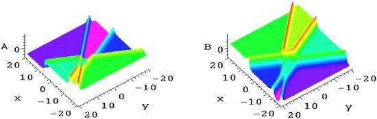
Figure 5. The interactions of the triple symmetry breaking solitons of A 3 and B 3 of the solution ( |
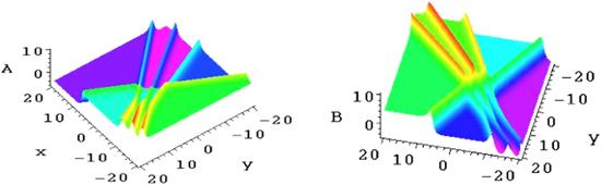
Figure 6. The interactions of the quadruple symmetry breaking solitons of A 4 and B 4 of the solution ( |
| • | • Symmetry breaking lump solution |
The lump solution is described by the rational function which is localized in all directions in the space. After a direct method proposed by Ma to obtain the lump solutions of the KP equation [35], the mixed lump-kink solutions to the KP equation and BKP equation [36, 37], the lump solutions to dimensionally reduced p-gKP and p-gBKP equations in (2+1)-dimensions [38] and a combined model of generalized bilinear KP and Bq equation [39], the rational lump solutions to a (2+1)-dimensional integrable KP equation with three arbitrary real constant coefficients [40] and a new (3+1)-dimensional generalized KP equation with constant coefficients [41] were presented successively. The lump structure for this AB–KP system (8 ) is constructed through the following long wave limit approach. After taking ${k}_{1}={\rho }_{1}{\varepsilon }_{1},{k}_{2}={\rho }_{2}{\varepsilon }_{2}$ , letting ${\delta }_{+}=-{\delta }_{-}$ and ${\varepsilon }_{1}\to 0,{\varepsilon }_{2}\to 0$ , equation (18 ) owns the expression $ \begin{eqnarray}\begin{array}{l}f={\rho }_{1}{\rho }_{2}\left[x-\displaystyle \frac{{x}_{0}}{2}+{l}_{1}\left(y-\displaystyle \frac{{y}_{0}}{2}\right)-\sigma {l}_{1}^{2}\left(t-\displaystyle \frac{{t}_{0}}{2}\right)\right]\\ \times \,\left[x-\displaystyle \frac{{x}_{0}}{2}+{l}_{2}\left(y-\displaystyle \frac{{y}_{0}}{2}\right)-\sigma {l}_{2}^{2}\left(t-\displaystyle \frac{{t}_{0}}{2}\right)\right]+\displaystyle \frac{12\beta {\rho }_{1}{\rho }_{2}}{\sigma {\left({l}_{1}-{l}_{2}\right)}^{2}}.\end{array}\end{eqnarray}$ One can verify that this solution satisfies the bilinear form (10 ). After putting the constant relations $ \begin{eqnarray}\begin{array}{rcl}{l}_{1} & = & \displaystyle \frac{{a}_{2}+{a}_{5}{\rm{i}}}{{\rho }_{1}},\ {l}_{2}=\displaystyle \frac{{a}_{2}-{a}_{5}{\rm{i}}}{{\rho }_{2}},\\ {\rho }_{1} & = & {a}_{1}+{a}_{4}{\rm{i}},\ {\rho }_{2}={a}_{1}-{a}_{4}{\rm{i}},\end{array}\end{eqnarray}$ with ${\rm{i}}$ is a unit of imaginary number, the following quadratic function f, which has been proved effectively to an integral equation, is reduced $ \begin{eqnarray}\begin{array}{rcl}f & = & {g}^{2}+{h}^{2}+{a}_{7},\ g={a}_{1}\left(x-\displaystyle \frac{{x}_{0}}{2}\right)+{a}_{2}\left(y-\displaystyle \frac{{y}_{0}}{2}\right)\\ & & +{a}_{3}\left(t-\displaystyle \frac{{t}_{0}}{2}\right),\\ h & = & {a}_{4}\left(x-\displaystyle \frac{{x}_{0}}{2}\right)+{a}_{5}\left(y-\displaystyle \frac{{y}_{0}}{2}\right)+{a}_{6}\left(t-\displaystyle \frac{{t}_{0}}{2}\right),\end{array}\end{eqnarray}$ where the real coefficients ${a}_{i}(i=1,2,\cdots ,7)$ have the relations $ \begin{eqnarray}\begin{array}{rcl}{a}_{3} & = & -\displaystyle \frac{({a}_{1}{a}_{2}^{2}-{a}_{1}{a}_{5}^{2}+2{a}_{2}{a}_{4}{a}_{5})\sigma }{{a}_{1}^{2}+{a}_{4}^{2}},\\ {a}_{6} & = & -\displaystyle \frac{({a}_{4}{a}_{5}^{2}-{a}_{4}{a}_{2}^{2}+2{a}_{1}{a}_{2}{a}_{5})\sigma }{{a}_{1}^{2}+{a}_{4}^{2}},\\ {a}_{7} & = & -\displaystyle \frac{3\beta {\left({a}_{1}^{2}+{a}_{4}^{2}\right)}^{3}}{{\left({a}_{1}{a}_{5}-{a}_{2}{a}_{4}\right)}^{2}\sigma }.\end{array}\end{eqnarray}$ The constraint conditions ${a}_{1}{a}_{4}\ne 0$ and ${a}_{1}{a}_{5}-{a}_{2}{a}_{4}\ne 0$ need to guarantee the rational analysis and localization of the functions $A,\ B$ of equation (9 ) in the (x, y)-plane. Therefore, the rational solutions of the AB–KP system (8 ) read $ \begin{eqnarray}\begin{array}{rcl}A & = & -\displaystyle \frac{48\beta {\left({a}_{1}g+{a}_{4}h\right)}^{2}}{\alpha {\left({g}^{2}+{h}^{2}+{a}_{7}\right)}^{2}}+\displaystyle \frac{24\beta ({a}_{1}^{2}+{a}_{4}^{2})}{\alpha ({g}^{2}+{h}^{2}+{a}_{7})}\\ & & +\displaystyle \frac{2a({a}_{3}g+{a}_{6}h)}{{g}^{2}+{h}^{2}+{a}_{7}}+\displaystyle \frac{2b({a}_{2}g+{a}_{5}h)}{{g}^{2}+{h}^{2}+{a}_{7}}\\ & & +\displaystyle \frac{2c\left({a}_{1}g+{a}_{4}h\right)}{{g}^{2}+{h}^{2}+{a}_{7}},\end{array}\end{eqnarray}$ $ \begin{eqnarray}\begin{array}{rcl}B & = & -\displaystyle \frac{48\beta {\left({a}_{1}g+{a}_{4}h\right)}^{2}}{\alpha {\left({g}^{2}+{h}^{2}+{a}_{7}\right)}^{2}}+\displaystyle \frac{24\beta ({a}_{1}^{2}+{a}_{4}^{2})}{\alpha ({g}^{2}+{h}^{2}+{a}_{7})}\\ & & -\displaystyle \frac{2a({a}_{3}g+{a}_{6}h)}{{g}^{2}+{h}^{2}+{a}_{7}}-\displaystyle \frac{2b({a}_{2}g+{a}_{5}h)}{{g}^{2}+{h}^{2}+{a}_{7}}\\ & & -\displaystyle \frac{2c\left({a}_{1}g+{a}_{4}h\right)}{{g}^{2}+{h}^{2}+{a}_{7}}.\end{array}\end{eqnarray}$ This set of rational solutions of equations (30 ) is a family of lump solutions for the functions g and h with $ \begin{eqnarray}\begin{array}{rcl}g & = & {a}_{1}\left(x-\displaystyle \frac{{x}_{0}}{2}\right)+{a}_{2}\left(y-\displaystyle \frac{{y}_{0}}{2}\right)\\ & & -\displaystyle \frac{({a}_{1}{a}_{2}^{2}-{a}_{1}{a}_{5}^{2}+2{a}_{2}{a}_{4}{a}_{5})\sigma }{{a}_{1}^{2}+{a}_{4}^{2}}\left(t-\displaystyle \frac{{t}_{0}}{2}\right),\end{array}\end{eqnarray}$ $ \begin{eqnarray}\begin{array}{rcl}h & = & {a}_{4}\left(x-\displaystyle \frac{{x}_{0}}{2}\right)+{a}_{5}\left(y-\displaystyle \frac{{y}_{0}}{2}\right)\\ & & -\displaystyle \frac{({a}_{4}{a}_{5}^{2}-{a}_{4}{a}_{2}^{2}+2{a}_{1}{a}_{2}{a}_{5})\sigma }{{a}_{1}^{2}+{a}_{4}^{2}}\left(t-\displaystyle \frac{{t}_{0}}{2}\right).\end{array}\end{eqnarray}$
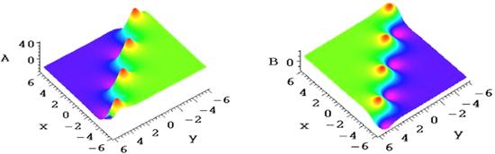
As a typical example, when taking the parameters $a=0,{a}_{1}=-2$ , ${a}_{2}={a}_{4}={a}_{5}=1$ , ${a}_{3}=-\tfrac{6}{5}$ , ${a}_{6}=-\tfrac{12}{5},{a}_{9}=\tfrac{125}{9},b=100$ , ${c}_{0}={x}_{0}={y}_{0}={t}_{0}=0$ , $\alpha =\tfrac{1}{5},\beta =1,\sigma =-3$ , the conditions ${a}_{1}{a}_{4}\ne 0$ and ${a}_{1}{a}_{5}-{a}_{2}{a}_{4}\ne 0$ are guaranteed. The corresponding symmetry breaking lumps are shown explicitly in figure 7 for the solutions A and B of equations (30 ). Figures 7 (a) and (b) are two three-dimensional plots of this symmetry lumps at time t = 0, figures 7 (c) and (d) are the corresponding density plots. Further, figures 8 and 9 are two density plots of the symmetry breaking lumps when the constant b = 15 and 2, respectively, while the others are invariant.
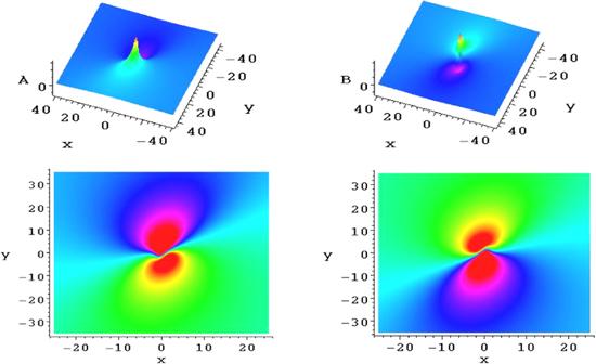
Figure 7. (a) and (b) are two three-dimensional plots of a pair of the symmetry breaking lumps of A and B of the solution ( |
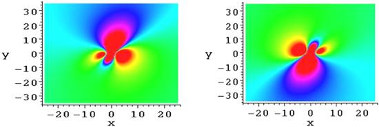
Figure 8. Two density plots of the symmetry breaking lumps of A and B of the solution ( |
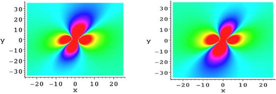
Figure 9. Two density plots of the symmetry breaking lumps of A and B of the solution ( |
The interaction solution of equations (8 ) between one lump soliton and the stripe soliton pairs is induced when the above quadratic function f combines with a hyperbolic cosine, that is $ \begin{eqnarray}\begin{array}{rcl}f & = & {g}^{2}+{h}^{2}+{a}_{7}+{k}_{0}\cosh \xi ,\\ g & = & {a}_{1}\left(x-\displaystyle \frac{{x}_{0}}{2}\right)+{a}_{2}\left(y-\displaystyle \frac{{y}_{0}}{2}\right)+{a}_{3}\left(t-\displaystyle \frac{{t}_{0}}{2}\right),\end{array}\end{eqnarray}$ $ \begin{eqnarray}\begin{array}{rcl}h & = & {a}_{4}\left(x-\displaystyle \frac{{x}_{0}}{2}\right)+{a}_{5}\left(y-\displaystyle \frac{{y}_{0}}{2}\right)+{a}_{6}\left(t-\displaystyle \frac{{t}_{0}}{2}\right),\\ \xi & = & {k}_{1}\left(x-\displaystyle \frac{{x}_{0}}{2}\right)+{k}_{2}\left(y-\displaystyle \frac{{y}_{0}}{2}\right)+{k}_{3}\left(t-\displaystyle \frac{{t}_{0}}{2}\right).\end{array}\end{eqnarray}$ The real coefficients ${a}_{i}(i=1,2,\cdots ,7)$ and ${k}_{i}(i=0,1,2,3)$ have the relations $ \begin{eqnarray}\begin{array}{rcl}{a}_{3} & = & -\displaystyle \frac{({a}_{1}{a}_{2}^{2}-{a}_{1}{a}_{5}^{2}+2{a}_{2}{a}_{4}{a}_{5})\sigma }{{a}_{1}^{2}+{a}_{4}^{2}},\\ {a}_{6} & = & -\displaystyle \frac{({a}_{4}{a}_{5}^{2}-{a}_{4}{a}_{2}^{2}+2{a}_{1}{a}_{2}{a}_{5})\sigma }{{a}_{1}^{2}+{a}_{4}^{2}},\\ {a}_{7} & = & -\displaystyle \frac{3\beta {\left({a}_{1}^{2}+{a}_{4}^{2}\right)}^{3}}{{\left({a}_{1}{a}_{5}-{a}_{2}{a}_{4}\right)}^{2}\sigma }-\displaystyle \frac{{k}_{0}^{2}{\left({a}_{1}{a}_{5}-{a}_{2}{a}_{4}\right)}^{2}\sigma }{12\beta {\left({a}_{1}^{2}+{a}_{4}^{2}\right)}^{3}},\end{array}\end{eqnarray}$ $ \begin{eqnarray}\begin{array}{rcl}{k}_{1} & = & \sqrt{-\displaystyle \frac{3\sigma }{\beta }}\displaystyle \frac{{a}_{1}{a}_{5}-{a}_{2}{a}_{4}}{3({a}_{1}^{2}+{a}_{4}^{2})},\\ {k}_{2} & = & \sqrt{-\displaystyle \frac{3\sigma }{\beta }}\displaystyle \frac{({a}_{1}{a}_{5}-{a}_{2}{a}_{4})({a}_{1}{a}_{2}+{a}_{4}{a}_{5})}{3{\left({a}_{1}^{2}+{a}_{4}^{2}\right)}^{2}},\\ {k}_{3} & = & -\displaystyle \frac{{k}_{1}^{4}\beta +{k}_{2}^{2}\sigma }{{k}_{1}}.\end{array}\end{eqnarray}$
The limited relations of the functions $g,h$ and $q\equiv {k}_{0}\cosh \xi $ are $ \begin{eqnarray}\begin{array}{l}\mathop{\mathrm{lim}}\limits_{t\to \pm \infty }\displaystyle \frac{g}{h}=\displaystyle \frac{{a}_{1}{a}_{2}^{2}-{a}_{1}{a}_{5}^{2}+2{a}_{2}{a}_{4}{a}_{5}}{{a}_{4}{a}_{5}^{2}-{a}_{4}{a}_{2}^{2}+2{a}_{1}{a}_{2}{a}_{5}},\mathop{\mathrm{lim}}\limits_{t\to \pm \infty }\displaystyle \frac{g}{q}=0,\\ \mathop{\mathrm{lim}}\limits_{t\to \pm \infty }\displaystyle \frac{h}{q}=0,\end{array}\end{eqnarray}$ which imply that two functions g and h are of the same order, while the hyperbolic cosine function q is higher when the time $t\to \pm \infty $ . Further, the function relation of g and ξ reads $ \begin{eqnarray}\begin{array}{rcl}\xi & = & \sqrt{-\displaystyle \frac{3\sigma }{\beta }}\displaystyle \frac{{a}_{1}{a}_{5}-{a}_{2}{a}_{4}}{3{a}_{1}({a}_{1}^{2}+{a}_{4}^{2})}g+\sqrt{-\displaystyle \frac{3\sigma }{\beta }}\displaystyle \frac{{a}_{4}{\left({a}_{1}{a}_{5}-{a}_{2}{a}_{4}\right)}^{2}}{3{a}_{1}{\left({a}_{1}^{2}+{a}_{4}^{2}\right)}^{2}}y\\ & & +\left[\sqrt{-\displaystyle \frac{3\sigma }{\beta }}\displaystyle \frac{({a}_{1}{a}_{5}-{a}_{2}{a}_{4})({a}_{1}{a}_{2}^{2}-{a}_{1}{a}_{5}^{2}+2{a}_{2}{a}_{4}{a}_{5})\sigma }{3{a}_{1}{\left({a}_{1}^{2}+{a}_{4}^{2}\right)}^{2}}\right.\\ & & \left.-\displaystyle \frac{{k}_{1}^{4}\beta +{k}_{2}^{2}\sigma }{{k}_{1}}\right]t.\end{array}\end{eqnarray}$ For this time, the resonance soliton pairs arise, because of ξ in equation (35 ) is a combination of the scaling and time displacement for the function g under the condition of g being a constant. According to equations (32 ) and (33 ), one can depict the interaction solution between one lump soliton and the stripe soliton pairs for the AB–KP system (8 ).
| • | • Symmetry breaking breather solution |
Based on the bilinear form (10 ) of the AB–KP system, the symmetry breaking breather solution of equations (8 ) can be expressed as [42, 43] $ \begin{eqnarray}\begin{array}{rcl}A & = & \displaystyle \frac{12\beta }{\alpha }{\left(\mathrm{ln}f\right)}_{{xx}}+a{\left(\mathrm{ln}f\right)}_{t}+b{\left(\mathrm{ln}f\right)}_{y}+c{\left(\mathrm{ln}f\right)}_{x},\\ B & = & A(-x+{x}_{0},-y+{y}_{0},-t+{t}_{0}),\end{array}\end{eqnarray}$ when the bilinear function $ \begin{eqnarray}\begin{array}{rcl}f & = & {b}_{1}\cosh \left[{k}_{1}\left(x-\displaystyle \frac{{x}_{0}}{2}\right)+{k}_{2}\left(y-\displaystyle \frac{{y}_{0}}{2}\right)+{k}_{3}\left(t-\displaystyle \frac{{t}_{0}}{2}\right)\right]\\ & & +{b}_{2}\cos \left[{k}_{4}\left(x-\displaystyle \frac{{x}_{0}}{2}\right)+{k}_{5}\left(y-\displaystyle \frac{{y}_{0}}{2}\right)+{k}_{6}\left(t-\displaystyle \frac{{t}_{0}}{2}\right)\right],\end{array}\end{eqnarray}$ and the relations of these coefficients $ \begin{eqnarray}{b}_{1}={b}_{2}\sqrt{-\displaystyle \frac{3{k}_{4}^{2}{\left({k}_{1}^{2}+{k}_{4}^{2}\right)}^{2}\beta -{\left({k}_{1}{k}_{5}-{k}_{2}{k}_{4}\right)}_{2}^{2}\sigma }{3{k}_{1}^{2}{\left({k}_{1}^{2}+{k}_{4}^{2}\right)}^{2}\beta +{\left({k}_{1}{k}_{5}-{k}_{2}{k}_{4}\right)}_{2}^{2}\sigma }},\end{eqnarray}$ $ \begin{eqnarray}\begin{array}{rcl}{k}_{3} & = & -{k}_{1}({k}_{1}^{2}-3{k}_{4}^{2})\beta -\displaystyle \frac{({k}_{1}{k}_{2}^{2}+2{k}_{2}{k}_{4}{k}_{5}-{k}_{1}{k}_{5}^{2})\sigma }{{k}_{1}^{2}+{k}_{4}^{2}},\\ {k}_{6} & = & -{k}_{4}(3{k}_{1}^{2}-{k}_{4}^{2})\beta -\displaystyle \frac{({k}_{4}{k}_{5}^{2}+2{k}_{1}{k}_{2}{k}_{5}-{k}_{4}{k}_{2}^{2})\sigma }{{k}_{1}^{2}+{k}_{4}^{2}}.\end{array}\end{eqnarray}$
Figure 10 is a pair of the symmetry breaking breather solitons when taking the constants $a=10$ , $b=c={x}_{0}\,={y}_{0}={t}_{0}=0$ , ${k}_{1}={k}_{2}={k}_{5}=\alpha =\beta =1$ , ${b}_{2}=\tfrac{1}{2},{k}_{4}=-1$ , $\sigma =-4$ , the others are ${b}_{1}=\tfrac{\sqrt{7}}{2},{k}_{3}=-2,{k}_{6}=6$ at time t = 0. For this time, the solutions A /B are $ \begin{eqnarray}\begin{array}{rcl}A/B & = & -\displaystyle \frac{12{[\sqrt{7}{\rm{\sinh }}({\xi }_{0})+{\rm{\sin }}({\eta }_{0})]}^{2}}{{[\sqrt{7}{\rm{\cosh }}({\xi }_{0})+{\rm{\cos }}({\eta }_{0})]}^{2}}\\ & & +\displaystyle \frac{12[\sqrt{7}{\rm{\cosh }}({\xi }_{0})-{\rm{\cos }}({\eta }_{0})]}{\sqrt{7}{\rm{\cosh }}({\xi }_{0})+{\rm{\cos }}({\eta }_{0})}\\ & & \mp \displaystyle \frac{10[\sqrt{7}{\rm{\sinh }}({\xi }_{0})+3{\rm{\sin }}({\eta }_{0})]}{\sqrt{7}{\rm{\cosh }}({\xi }_{0})+{\rm{\cos }}({\eta }_{0})},\end{array}\end{eqnarray}$ with ${\xi }_{0}=x+y-2t$ and ${\eta }_{0}=-x+y+6t$ . This set of special solutions A /B are the combination of the trigonometric functions sin/cos and hyperbolic functions sinh/cosh. The property of these functions determines the symmetry breaking breather structures. That is, the solitary wave determined by the hyperbolic functions with the variable ${\xi }_{0}$ , while the periodic wave comes from the trigonometric functions with the variable ${\eta }_{0}$ . The propagating speed of the solitary wave is −2 in x /y -axis and the periodic wave is −6 in x -axis, but 6 in y -axis. From figure 10, one can see clearly that the periodicity moves along the propagation direction while the localization also along the straight line $x+y=0$ for the time t = 0.
Figure 10. A pair of the symmetry breaking breather solitons of A and B of the solution ( |
4. Summary and discussion
We know that the soliton structures are the fundamental local excitations. The explicit full reversal symmetries including parity, time reversal, soliton initial position reversal and charge conjugate reversal are convenient in the studies on the nonlinear physical problems, such as the multi-place nonlocal systems and the resonant structures [18, 19, 44]. The AB systems were proposed by Lou through the symmetry of the shifted parity, time reversal and charge conjugation to describe two correlated events [11 –13]. In this paper, the coupled AB system (7 ) of the KP equation (5 ) is first established. This two-place physical AB–KP system possesses nonlocal ${\hat{P}}_{s}^{x}{\hat{P}}_{s}^{y}{\hat{T}}_{d}$ symmetry, that is, the system is invariant under the transformation $\{x\to -x+{x}_{0}$ , $y\to -y+{y}_{0},t\to -t+{t}_{0}\}$ . By introducing an extended Bäcklund transformation (9 ) and its Hirota bilinear formation (10 ), the symmetry breaking multisoliton solutions (9 ) with (13 ) of equations (8 ), including the line soliton solution (16 ), the interaction of the double line solitons (17 ) and the interactions of the multifold solitons (22 ) and (23 ), are presented successively. The rational lump solution (30 ) for the AB–KP system (8 ) arises from the long wave limit of equation (18 ), while the interaction solution between one lump soliton and the stripe soliton pairs is induced when the quadratic function f combine with a hyperbolic cosine. Finally, with the aid of the property of the trigonometric function and hyperbolic function, the symmetry breaking breather solution (36 ) is constructed. Almost all of these explicit solutions are depicted the symmetry breaking structures with some special constants.
In fact, there are still some open problems should be investigated. One can derive more special solutions for equations (8 ) which may produce other local and nonlocal structures, such as symmetry breaking cnoidal wave and rogue wave. The algebraic structures, such as Lie point symmetry and symmetry reduction, Bäcklund transformation related to residual symmetry may also be achieved strictly for equations (8 ). Finally, the ${\hat{P}}_{s}^{x}{\hat{P}}_{s}^{y}{\hat{T}}_{d}$ symmetry of this paper for an integral system could be deeply studied through taken one of the elements of the eight order ${\hat{P}}_{s}{\hat{T}}_{d}\hat{C}$ group [21, 24] $ \begin{eqnarray}{\rm{\Theta }}=\{I,\,\hat{C},\,{\hat{P}}_{s}^{x}{\hat{T}}_{d},\,{\hat{P}}_{s}^{y},\,{\hat{P}}_{s}^{x}{\hat{T}}_{d}\hat{C},\,{\hat{P}}_{s}^{y}\hat{C},\,{\hat{P}}_{s}^{x}{\hat{P}}_{s}^{y}{\hat{T}}_{d},\,{\hat{P}}_{s}^{x}{\hat{P}}_{s}^{y}{\hat{T}}_{d}\hat{C}\},\end{eqnarray}$ where the operators ${\hat{P}}_{s}^{x}$ , ${\hat{P}}_{s}^{y}$ , ${\hat{T}}_{d}$ and $\hat{C}$ are defined by $ \begin{eqnarray}\begin{array}{l}{\hat{P}}_{s}^{x}x=-x+{x}_{0},\,{\hat{P}}_{s}^{y}y=-y+{y}_{0},\\ \quad {\hat{T}}_{d}t=-t+{t}_{0},\,\hat{C}A={A}^{* }.\end{array}\end{eqnarray}$