Investigating the dynamic characteristics of nonlinear models that appear in ocean science plays an important role in our lifetime. In this research, we study some features of the paired Boussinesq equation that appears for two-layered fluid flow in the shallow water waves. We extend the modified expansion function method (MEFM) to obtain abundant solutions, as well as to find new solutions. By using this newly modified method one can obtain novel and more analytic solutions comparing to MEFM. Also, numerical solutions via the Adomian decomposition scheme are discussed and favorable comparisons with analytical solutions have been done with an outstanding agreement. Besides, the instability modulation of the governing equations are explored through the linear stability analysis function. All new solutions satisfy the main coupled equation after they have been put into the governing equations.
Hajar Farhan Ismael, Hasan Bulut, Haci Mehmet Baskonus, Wei Gao. Newly modified method and its application to the coupled Boussinesq equation in ocean engineering with its linear stability analysis[J]. Communications in Theoretical Physics, 2020, 72(11): 115002. DOI: 10.1088/1572-9494/aba25f
1. Introduction
Studies on the dynamics of multiple nonlinear evolution equations over the past two centuries have caught the attention of many researchers across the globe. Nonlinear evolution equations are used in the study of complex nonlinear features that explain many of our true-life problems in different areas of nonlinear science, like the modeling of interactions between atmospheric and oceanic factors, optical fibers, nonlinear dynamics, fluid dynamics, and plasma physics. It is also very important to discuss the characteristics of models that occur in ocean dynamics due to the key positions they perform in our day-to-day operations or activities. Because of the applications and rules that NLODEs carry out in our everyday lives, researchers around the world have used a variety of numerical and analytical methods to explore their behaviors, such as the Adomian decomposition method [1 –3], a semi-implicit method and a finite element method [4], the finite difference method [5, 6], a shooting method [7 –9], a homotopy perturbation method [10], a modified expansion method [11 –13], the sinh-Gordon expansion method [14 –16], the sin-Gordon expansion method [17 –19], an improved tan $\left(\phi \left(\xi \right)/2\ \right)$ [20 –22], an inverse mapping method [23], the Bäcklund transformation [24], a functional variable method [25], a $\left(m+\left(G^{\prime} /G\right)\right)$ -expansion method [26, 27], a modified auxiliary expansion method [28], the Jacobi elliptic function method [29, 30], the improved Bernoulli sub-equation function method [31, 32], the Riccati–Bernoulli sub-ODE method[33, 34], a $\left(1/G^{\prime} \ \right)$ -expansion method [35, 36], and many other numerical and exact techniques [37 –43].
Peregrin [44] first reported the Boussinesq equations for variable water depth, which are efficient for shallow water, as well as linked to it as a normal Boussinesq equation. Boussinesq equations are the most common nonlinear partial differential equations developed to describe water dynamics with both a low amplitude as well as a long wave. Such equations are one of the most important equations for forecasting wave changes in coastal regions, as well as commonly used in coastal and ocean engineering. In this research, we use the newly modified expansion function method (MEFM) to find new solutions for the Boussinesq-type equations and the Adomian decomposition method to studies numerical solutions to the suggested equations. Moreover, the instability modulation of models is also presented.
The Boussinesq equations in (1+1)-dimensions [45] are read
This paired Boussinesq equation also appears in shallow water waves for two layers of fluid flow. This scenario occurs at a time when accidental oil spills from a vessel, resulting in a layer of oil floating above the water surface.
2. General structures of the method
Suppose there is a nonlinear partial differential equation
where ai, bj, ci and dj, $\left(0\leqslant i\leqslant n,0\leqslant j\leqslant m\right)$ are constants and $\phi \left(\xi \right)$ is the auxiliary ODE defined by
according to the balanced relationship between $V^{\prime\prime} $ and V3, we get n = m + 1, choosing m = 1 gives n = 2. Substituting the value of n and m into equation (5 ) yields
Using equation (12 ) and its second derivative with equation (11 ), we gain the polynomial equation of ${a}^{\phi \left(\xi \right)}$ . After that, we obtain a set of algebraic equations from this polynomial by matching the sum of the ${a}^{\phi \left(\xi \right)}$ coefficients with the same power to zero. By solving the system of equations, we can obtain and study the following solutions.
Case 1. When ${a}_{0}={b}_{0}\left(-\lambda +\sqrt{{\rm{\Delta }}}\right)$, ${a}_{1}=-\tfrac{{b}_{0}{c}_{0}}{{d}_{1}}\,+{b}_{1}\left(-\lambda +\sqrt{{\rm{\Delta }}}\right)$, ${a}_{2}=-\tfrac{{b}_{1}{c}_{0}}{{d}_{1}}$, ${c}_{2}=-2{d}_{1}\mu $, $k=\sqrt{{\rm{\Delta }}},{d}_{0}=0,{c}_{1}=0$, we get the following solutions:
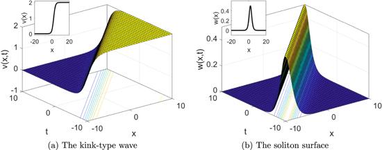
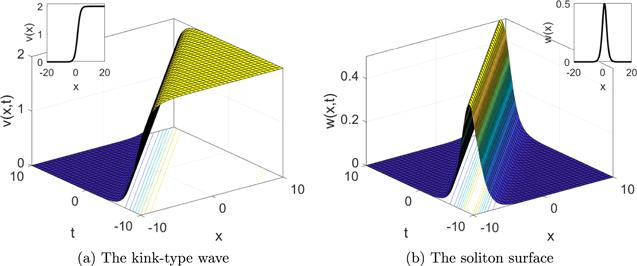
providing that ${\rm{\Delta }}={\lambda }^{2}-4\mu \gt 0$, $\lambda \ne 0,\mu \ne 0$ . Equations (13 ) and (14 ) are the kink-type and soliton surfaces as seen in figure 1 .
Figure 1. 3D and 2D graph of equations (13 ) and (14 ) drawn when λ = 3, μ = 2, ε = 0.1.
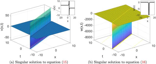
Case 2. When ${a}_{0}={b}_{0}\left(\lambda +2\sqrt{{\rm{\Delta }}}\right)$, ${a}_{1}={b}_{0}\left(-2-\tfrac{{c}_{0}}{{d}_{1}}+\tfrac{\lambda \left(\lambda +\sqrt{{\rm{\Delta }}}\right)}{\mu }\right)$, ${a}_{2}=-\tfrac{{b}_{0}{c}_{0}\lambda }{2{d}_{1}\mu }$, ${c}_{2}=2{d}_{1}\mu ,{b}_{1}=\tfrac{{b}_{0}\lambda }{2\mu }$, $k=2\sqrt{{\rm{\Delta }}},{d}_{0}=0,{c}_{1}=0$, we get the following singular solutions (see figure 2 ):
Figure 2. 3D and 2D graph of equations (15 ) and (16 ) drawn when λ = 3, μ = 2, ε = 1.
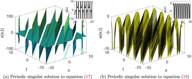
Case 3. When ${a}_{0}={b}_{0}k+\tfrac{\sqrt{-{{b}_{0}}^{2}\left({k}^{2}-8\mu \right)}}{\sqrt{2}}$, ${a}_{1}=\tfrac{1}{4}\left({b}_{0}\left(8-\tfrac{4{c}_{0}}{{d}_{1}}\right)+\tfrac{\sqrt{2}k\sqrt{-{{b}_{0}}^{2}\left({k}^{2}-8\mu \right)}}{\mu }\right)$, ${a}_{2}=-\tfrac{{c}_{0}\sqrt{-{{b}_{0}}^{2}\left({k}^{2}-8\mu \right)}}{2\sqrt{2}{d}_{1}\mu }$, ${c}_{2}=2{d}_{1}\mu $, ${d}_{0}=0,{c}_{1}=0,{b}_{1}=\tfrac{\sqrt{-{{b}_{0}}^{2}\left({k}^{2}-8\mu \right)}}{2\sqrt{2}\mu },\lambda =\tfrac{\sqrt{-{{b}_{0}}^{2}\left({k}^{2}-8\mu \right)}}{\sqrt{2}{b}_{0}}$, we have the following periodic singular solutions (see figure 3 ):
Figure 3. 3D and 2D graph of equations (17 ) and (18 ) drawn when ε = 0.1, k = 1.
Case 4. When ${a}_{1}={b}_{1}k+\sqrt{{{b}_{1}}^{2}\left({k}^{2}+4\mu \right)}$, ${a}_{2}=2{b}_{1},{c}_{1}=-\tfrac{{a}_{0}{d}_{0}}{{b}_{1}}$, ${c}_{2}=-\tfrac{{a}_{0}{d}_{1}}{{b}_{1}}$, $\lambda =\tfrac{\sqrt{{{b}_{1}}^{2}\left({k}^{2}+4\mu \right)}}{b1}$, ${c}_{0}=0,{b}_{0}=0$, we can construct and study the following solutions:
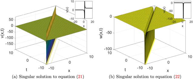
Solution 1. In case ${\lambda }^{2}-4\mu \gt 0,\mu \ne 0,\lambda \ne 0$, we get
Figure 5. 3D and 2D graph of equations (21 ) and (22 ) drawn when $\mu =0,\epsilon =0.1,k=1,{b}_{1}=0.1$ .
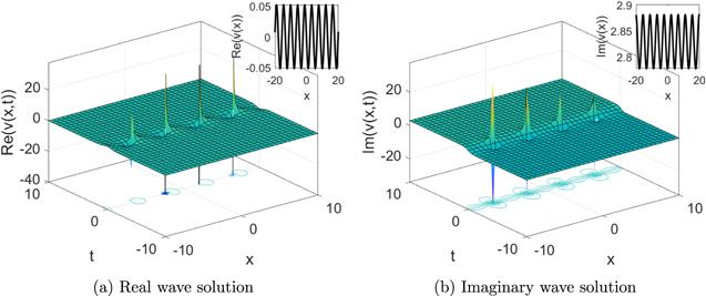
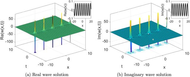
Case 5. When ${c}_{0}=-\tfrac{{a}_{2}{d}_{1}}{{b}_{1}}$, ${c}_{1}=-\tfrac{{d}_{1}\left({a}_{1}+\left(1-{\rm{i}}\sqrt{2}\right){b}_{1}\lambda \right)}{{b}_{1}}$, ${c}_{2}=-\tfrac{{a}_{0}{d}_{1}}{{b}_{1}}-\tfrac{3{d}_{1}{\lambda }^{2}}{2}$, $k={\rm{i}}\sqrt{2}\lambda $, $\mu =\tfrac{3{\lambda }^{2}}{4},{d}_{0}=0,{b}_{0}=0$ and ${\lambda }^{2}-4\mu \lt 0$, we can construct the below solutions
Equations (23 ) and (24 ) are complex solutions to the studied equations as seen in figures 6 and 7, respectively.
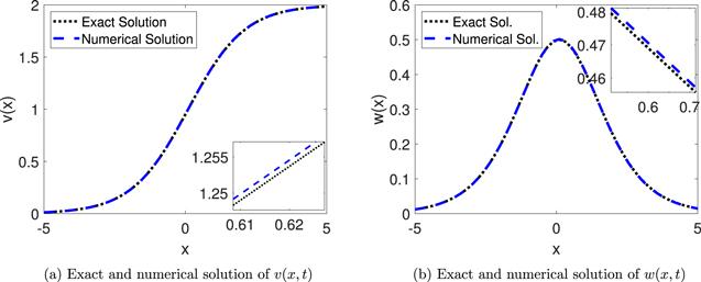
4. Numerical solutions
In this portion of work, we study the numerical solutions of equation (1 ) by using the Adomian decomposition scheme. Consider the (1+1)- dimensional Boussinesq equations in equation (1 ), and rewrite it as below
where $L=\tfrac{\partial }{\partial t}$ . Now from equations (13 ) and (14 ), one can find initial conditions that cover the equations (25 ) and (26 ) as shown below
Defining the inverse operator ${L}^{-1}\left(* \right)={\int }_{0}^{t}\left(* \right)\ {\rm{d}}{t}$ and applying it on equations (25 ) and (26 ), we have
where ${A}_{i},{B}_{i},{C}_{i}$ are the Adomian polynomial of ${v}_{k},{w}_{k}$ . Plugging equation (33 ) into equations (31 ) and (32 ), the first-two terms of solutions can be written as follows
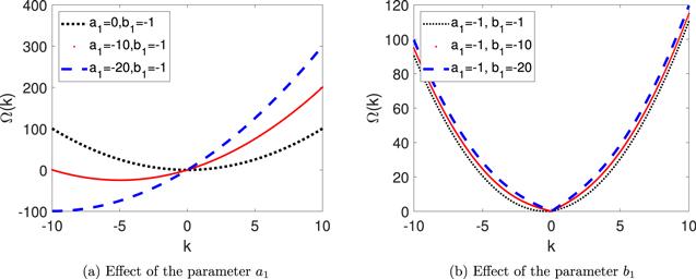
Figure 9. Frequency of the perturbation versus the wave number.
Table 1. Analytical and numerical solutions of v (x, t) for the equation (1 ) and its absolute errors when λ = 3, μ = 2, ε = 0 under equation (13 ).
xi
ti
Exact solution
Numerical solution
Absolute error
0.01
0.1
0.9550303504
0.954955901
7.44484 × 10⁻⁵
0.02
0.1
0.9600213196
0.959960033
6.12866 × 10⁻⁵
0.03
0.1
0.9650142846
0.964966309
4.79749 × 10⁻⁵
0.04
0.1
0.9700089967
0.969974480
3.45162 × 10⁻⁵
0.05
0.1
0.9750052070
0.974984293
2.09135 × 10⁻⁵
0.06
0.1
0.9800026662
0.979995496
7.1697 × 10⁻⁶
0.07
0.1
0.9850011248
0.985007836
6.7119 × 10⁻⁶
0.08
0.1
0.9900003333
0.990021061
2.07283 × 10⁻⁵
0.09
0.1
0.9950000416
0.995034917
3.48762 × 10⁻⁵
Table 2. Analytical and numerical solutions of w (x, t) for the equation (1 ) and its absolute errors when λ = 3, μ = 2, ε = 0 under equation (14 ).
xi
ti
Exact solution
Numerical solution
Absolute error
0.01
0.1
0.4989888653
0.5002974576
1.3085923 × 10⁻³
0.02
0.1
0.4992008525
0.5005245744
1.3237219 × 10⁻³
0.03
0.1
0.4993879998
0.5007265680
1.3385682 × 10⁻³
0.04
0.1
0.4995502698
0.5009033929
1.3531231 × 10⁻³
0.05
0.1
0.4996876301
0.5010550088
1.3673786 × 10⁻³
0.06
0.1
0.4998000533
0.5011813804
1.3813270 × 10⁻³
0.07
0.1
0.4998875168
0.5012824775
1.3949606 × 10⁻³
0.08
0.1
0.4999500033
0.5013582752
1.4082719 × 10⁻³
0.09
0.1
0.4999875002
0.5014087537
1.4212535 × 10⁻³
5. Linear stability analysis to the coupled Boussinesq equation
In this portion, the notion of linear stability analysis will be used to explore and study the stability analysis of the coupled Boussinesq equation. Assume that the perturbed solutions have the forms [46, 47]:
where ${a}_{1},{b}_{1}$ describe the steady-state solutions for equation (1 ) and a2, b2 are constants. Putting equations (40 ) and (41 ) into equation (1 ) and making the linearization, the results yield:
due to this result, we investigate the linear stability of coupled Boussinesq equations that is dependent on the values of steady-state parameters a1, b1 . The effects of these parameters are presented graphically as shown in figure 9 . From equation (50 ), we observe that the real part will be negative in condition k > 0, therefore the dispersion is unstable while the situation will become stable when k < 0 as well as it occurs if a1 < 0. In the case, a1 = 0 the dispersion is called marginally stable, which is occur when the real part is equal to zero.
6. Results and discussion
In this work, we are newly extended the MEFM to analyze and study some new solutions for partial differential equations. Applying this newly modified method on the studied equations leads to the new solutions, as well as gives us a more exact solutions, too. We have successfully applied this newly modified method to couple Boussinesq equation, and the results lead to new the solutions. The MEFM has been successfully implemented to the couple Boussinesq equation in [48], and two cases of the solutions are revealed. In this paper, the solutions observed in equations (13 )–(16 ), and equations (21 ), (22 ) are the same, but the solutions constructed in equations (17 ), (18 ), and complex solutions (23 ), (24 ) are novel and successfully constructed via this method. This approach is straightforward, reliable, and easy-to-use as a mathematical tool that can be applied to other nonlinear models or nonlinear partial differential equations to study and depict real and complex solutions.
7. Conclusion
In this article, the paired Boussinesq equation that occurs for two-layered fluid flow in the shallow water waves is solved analytically and numerically. The modified expansion function method is improved to investigate some new exact solutions, as well as the Adomian decomposition method is used to investigate numerical solutions. All solutions are novel and distinct from those obtained by using MEFM, meanwhile by using this method we can reveal more analytical solutions compared to MEFM. The topological kink-type waves, soliton surfaces, periodic singular, and some new types of singular solutions are presented. All newly gained exact solutions are also plotted in 2D and 3D together with a contour plot. Comparison between the new exact proposed solutions and the numerical solutions are also discussed. Besides, the instability modulation is investigated through the linear stability analysis method for the governing equations. All the solutions found are inserted into the studied equations, and they are satisfied.


