


1. Introduction
Nonlinear evolution equations, which depend on certain space–time signatures, have a multitude of important applications across broad disciplines including physics, finance and biology. Certain special solutions to such equations can exhibit soliton behaviors, that is, they do not disperse and thus conserve their original forms after the collision [1]. Moreover, interaction between solitons is one of the most fascinating features of many soliton phenomena [2].
While direct numerical solutions to some evolution equations are computationally expensive, with the revival of deep learning, it has attracted much interest on the development of more efficient data-driven solutions to nonlinear evolution equations [3 –5]. As a direction of machine learning, deep learning methods are able to effectively learn the feature representations from raw data [6 –10]. However, to our knowledge, previous works focus mainly on some simple solutions to the given equations, which could not uncover the soliton behaviors under some circumstances. Thus, we propose to combine a neural network framework with some underlying physical laws to reconstruct the soliton solutions.
For a certain amount of physical systems, some nonlinear and dispersive processes compete while the dissipation can be neglected. Therefore, in this paper, we will study nonlinear time-dependent partial differential equations where each contains the dispersive term in addition to other partial derivatives. These equations often play important roles in many scientific applications and physical phenomena. Specifically, we consider the (1 + 1)-dimensional third-order nonlinear evolution equations of the form $ \begin{eqnarray}{u}_{t}={ \mathcal N }(u,{u}_{x},{u}_{{xx}},{u}_{{xxx}}),\end{eqnarray}$ in order to solve their soliton solutions, where the subscripts t and x denote the partial derivatives with respect to them and ${ \mathcal N }$ is a nonlinear function of the solution u and its arbitrary-order partial derivatives with respect to the spatial variable x (concretely, in this work, the highest order is three).
Consequently, define the residual network $ \begin{eqnarray}f:= {u}_{t}-{ \mathcal N }(u,{u}_{x},{u}_{{xx}},{u}_{{xxx}}),\end{eqnarray}$ and then the solution network is trained to satisfy the residual constraint (2 ), which plays a role of regularization and is embedded into the mean-squared objective function [16] $ \begin{eqnarray}L=\displaystyle \frac{1}{{N}_{u}}\displaystyle \sum _{i=1}^{{N}_{u}}| u({t}_{u}^{i},{x}_{u}^{i})-{u}^{i}{| }^{2}+\displaystyle \frac{1}{{N}_{f}}\displaystyle \sum _{j=1}^{{N}_{f}}| f({t}_{f}^{j},{x}_{f}^{j}){| }^{2}.\end{eqnarray}$
In this work, we choose the network architecture in a consistent fashion [17]. Specifically, we learn the unknown solution u by using a 13-layer feedforward network with 40 neurons per hidden layer. For the choice of activation functions, we have conducted many experiments for different functions such as tanh, sin, sigmoid (σ) and rectified linear units (ReLU) in different number of layers and neurons. We find that the tanh function is a little unstable. Moreover, the results indicate that the σ and ReLU functions could not represent the data in current settings. So we select sin as the activation function in most cases. In addition, we just tune all parameters of the objective (3 ) using the L-BFGS method [18]. More modern and efficient algorithms can be adopted for larger-scale data, for example, Adam [19], which is a variant of the stochastic gradient descent algorithm. All numerical examples reported here are run on a MacBook Pro computer with 2.4 GHz Dual-Core Intel Core i5 processor and 8 GB memory.
The outline of this paper follows. In section 2 , we reconstruct the one-soliton and two-soliton solutions to the KdV equation from data collected from simulations. Consequently, we recover the one-soliton and breather solutions to the mKdV equation in section 3 . In section 4 , we then consider the kink solution to the KdV–Burgers equation. In section 5 , we focus mainly on the soliton fusion and fission phenomena of the STO equation. Finally, some concluding discussion and remarks are contained in section 6 .
2. The KdV equation
The KdV equation [20, 21] is a canonical model which describes the unidirectional propagation of shallow water waves with certain small amplitude and long wavelength. It also is one of the earliest equations with soliton solutions. The KdV equation can be regarded as a dispersive modification of the Burgers equation and converted by the Cole–Hopf transformation. The dispersion and nonlinearity of this equation balance each other which leads to the wave propagation without losing energy. However, The manifestation of the balance may vary from system to system, thus other evolution equations could have different soliton forms from the KdV equation whose soliton solutions are bell-shaped.
In this section, we consider the KdV equation along with Dirichlet boundary conditions [22 –24] given by $ \begin{eqnarray}\left\{\begin{array}{l}{u}_{t}+6{{uu}}_{x}+{u}_{{xxx}}=0,x\in [-20,20],t\in [-5,5],\\ u({t}_{0},x)={u}_{0}(x),\\ u(t,-20)=u(t,20)=0,\end{array}\right.\end{eqnarray}$ where u 0 (x) is an arbitrary real-valued function. In this case, ${ \mathcal N }=-6{{uu}}_{x}-{u}_{{xxx}}$ .
Note that this equation and the mKdV equation which will be considered in the next section are both special cases of the generalized KdV equation
$ \begin{eqnarray*}{u}_{t}+{u}_{{xxx}}+{\left({u}^{p}\right)}_{x}=0,\end{eqnarray*}$
where the case p = 2 obviously corresponds to the KdV equation and p = 3 to the mKdV equation. By the way, these two equations are completely integrable.
where the case p = 2 obviously corresponds to the KdV equation and p = 3 to the mKdV equation. By the way, these two equations are completely integrable.
2.1. One-soliton solution
Here, we first consider the one soliton problem. Some exact soliton solutions to such nonlinear evolution equations can be expressed in terms of elementary functions and then these solutions are very important for understanding the nonlinearity of these systems better. Meanwhile, they are also useful in testing the performance and accuracy of certain numerical methods. Applying some analytic methods [25, 26], one can show that the exact one-soliton solution to equation (4 ) admits the explicit expression given by
$ \begin{eqnarray*}u(t,x)=\displaystyle \frac{c}{2}{{\rm{sech}} }^{2}\left(\displaystyle \frac{\sqrt{c}}{2}(x-{x}_{0}-{ct})\right).\end{eqnarray*}$
Specifically, we just set c = 3 for convenience. Then, the corresponding initial condition is obtained with a specific initial displacement by $ \begin{eqnarray}{u}_{0}(x)=\displaystyle \frac{3}{2}{{\rm{sech}} }^{2}\left(\displaystyle \frac{\sqrt{3}}{2}(x+15)\right).\end{eqnarray}$
We simulate equation (4 ) using the conventional spectral method to obtain the data. Specifically, starting from the initial condition (5 ), we use the Chebfun package [27] with a Fourier spatial discretization with 512 modes and a 4th-order explicit Runge–Kutta (RK) integrator with time-step size 1 × 10− 4, and then integrate the equation up to the final instant t = 5. The solution is saved every Δt = 0.05 to give us totally 201 snapshots. We generate a smaller training dataset out of this data by randomly sub-sampling N u = 100 initial-boundary data and N f = 10 000 collocation points which are generated by the Latin hypercube sampling method [28].
Figure 1 demonstrates our result for the data-driven one-soliton solution to the KdV equation (4 ). Specifically, given a set of initial and boundary data points, we try to learn the latent solution u (t, x) by tuning all learnable parameters of the network using the loss function (3 ). The top panel of figure 1 compares between the exact solution and the predicted spatiotemporal solution. The model achieves a relative ${{\mathbb{L}}}_{2}$ error of size 3.44 × 10⁻³ in a runtime of approximately three and half a minute. We can see a more detailed assessment in the bottom panel of figure 1 . We particularly present a comparison between the exact solution and the predicted solutions at different times t = −3.75, −1.25, 3.75. The algorithm accurately reconstructs the one-soliton solution to the KdV equation.
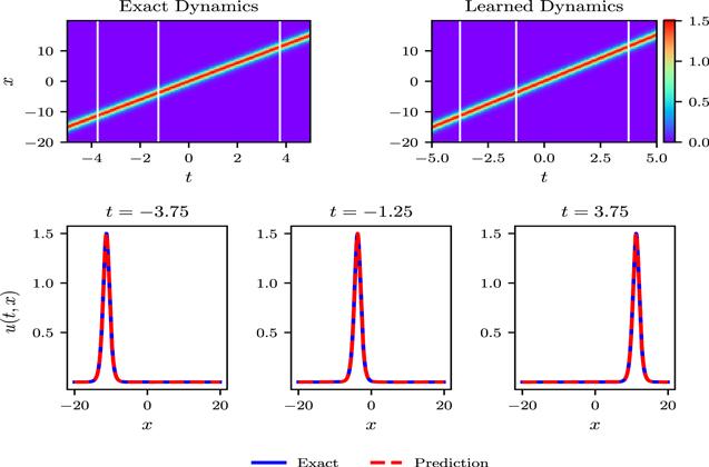
Figure 1. The KdV equation. Top: a one-soliton solution to the KdV equation (left panel) is compared to the corresponding predicted solution to the learned equation (right panel). The network correctly captures the dynamics behavior and accurately reproduces the soliton solution with a relative |
From figure 2, we can observe the reconstructed single solitary wave motion better.
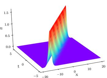
Figure 2. The spatiotemporal behavior of a one-soliton solution to the learned KdV equation. |
2.2. Two-soliton solutions
Many non-integrable equations also possess localized shape-preserving traveling waves that resemble soliton solutions. For example, it would be indistinguishable from a KdV soliton to single traveling wave solution of the wave equation expressed by
$ \begin{eqnarray*}{u}_{t}+{u}_{x}=0.\end{eqnarray*}$
However, only integrable ones have the universal property of possessing several exact multi-soliton solutions which reflect perfectly nonlinear elastic interactions between individual solitons. Thus, we now consider the two-soliton problem [26] as an example. Using certain similar analytical methods, the exact two-soliton solution to equation (4 ) is given by
$ \begin{eqnarray*}\begin{array}{rcl}u(t,x) & = & \displaystyle \frac{{c}_{1}}{2}{{\rm{sech}} }^{2}\left(\displaystyle \frac{\sqrt{{c}_{1}}}{2}(x-{x}_{1}-{c}_{1}t)\right)\\ & & +\displaystyle \frac{{c}_{2}}{2}{{\rm{sech}} }^{2}\left(\displaystyle \frac{\sqrt{{c}_{2}}}{2}(x-{x}_{2}-{c}_{2}t)\right),\end{array}\end{eqnarray*}$
where c 1 and c 2 denote the speeds of two individual solitons, respectively. From this expression, we know that the width of the soliton is inversely proportional to the square root of the wave speed for the KdV equation. Assuming${c}_{1}\gg {c}_{2}$ without loss of generality, if such two solitons are well separated with the taller (and thus narrower) to the left of the shorter, then the taller soliton travels faster to the right and would interact nonlinearly and collide elastically with the shorter one [1, 29, 30].
where c 1 and c 2 denote the speeds of two individual solitons, respectively. From this expression, we know that the width of the soliton is inversely proportional to the square root of the wave speed for the KdV equation. Assuming
As an example, an initial solution is given explicitly by $ \begin{eqnarray}{u}_{0}(x)=\displaystyle \frac{3}{2}{{\rm{sech}} }^{2}\left(\displaystyle \frac{\sqrt{3}}{2}(x+15)\right)+\displaystyle \frac{1}{2}{{\rm{sech}} }^{2}\left(\displaystyle \frac{1}{2}(x+3)\right).\end{eqnarray}$
Using the above same spectral method, starting from the initial condition (6 ), we use the Chebfun package [27] with a Fourier spatial discretization with 512 modes and a 4th-order explicit RK integrator with time-step size 1 × 10⁻⁴, and then integrate the equation up to the final instant t = 5. The solution is saved every Δt = 0.05 to give us totally 201 snapshots. We generate a smaller training dataset out of this data by randomly sub-sampling N u = 100 initial-boundary data and N f = 10 000 collocation points.
Figure 3 demonstrates the evolution of two KdV solitons with different amplitudes, which enables the unique determination of the governing equation [31]. Specifically, given a set of initial and boundary data points, we try to learn the unknown solution u (t, x) by training the network using the loss function (3 ). The top panel of figure 3 compares between the exact dynamics and the predicted solution. Initially, we have two clearly separated solitons. Then, they lose their identities in certain sort and merge into a composite structure during the interaction. Numerical simulations of the process show that a lower wave hump is formed in the interaction region. The result indicates that it is a nonlinear superposition of shifted counterparts which distinguishes from some other simple solitary traveling waves. After a while, these two solitons emerge from the interaction again. The model achieves a relative ${{\mathbb{L}}}_{2}$ error of size 7.39% in a runtime of approximately half an hour. We can see a more detailed assessment of the predicted solution in the bottom panel of figure 3 . We present a comparison between the exact solutions and the predicted solutions at different instants t = −3.75, −1.25, 3.75. From the bottom of figure 3, we see that the wave patterns they produced match with the exact solutions well.
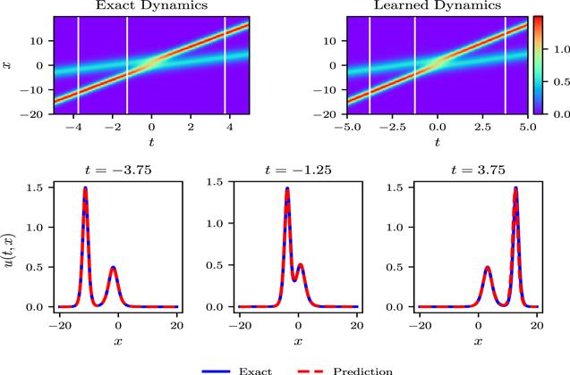
Figure 3. The KdV equation. Top: a two-soliton solution to the KdV equation is compared to the corresponding predicted solution to the learned equation (right panel). The model correctly exhibits the dynamics behavior and accurately reproduces the solution with a relative |
From figure 10, we can observe the elastic collision of two individual solitons with different amplitudes better.
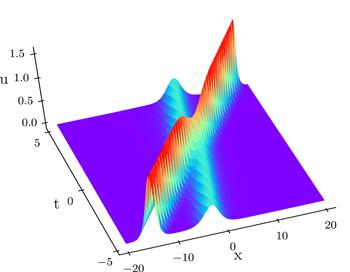
Figure 4. The spatiotemporal behavior of a two-soliton solution to the learned KdV equation. |
In addition, if the speeds of these two solitons are close, i.e. $0\lt \tfrac{{c}_{1}-{c}_{2}}{{c}_{1}+{c}_{2}}\ll 1$ , the solitons will exchange their sizes and speeds at certain much long distance and consequently avoid the collision [32]. For instance, we consider the initial condition $ \begin{eqnarray}\begin{array}{rcl}{u}_{0}(x) & = & \displaystyle \frac{1.01}{2}{{\rm{sech}} }^{2}\left(\displaystyle \frac{\sqrt{1.01}}{2}(x+12)\right)\\ & & +\displaystyle \frac{1}{2}{{\rm{sech}} }^{2}\left(\displaystyle \frac{1}{2}(x-2)\right),\end{array}\end{eqnarray}$ and adopt the same data generation and sampling method.
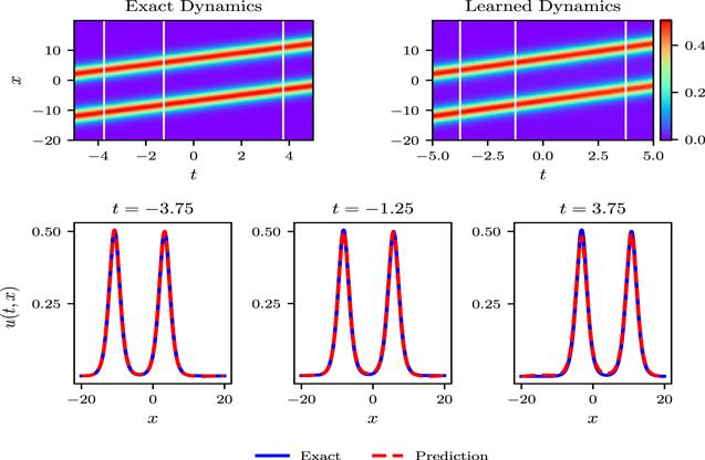
Figure 5. The KdV equation. Top: another two-soliton solution to the KdV equation (left panel) is compared to the predicted solution to the learned equation. The model correctly exhibits the dynamics behavior and accurately reproduces the solution with a relative |
3. The mKdV equation
The mKdV equation, which can be regarded as the KdV equation with a cubic nonlinearity, is also an integrable model that possesses most of the properties of the KdV equation [34 –39] and even has a richer family of solutions including breathers. By the way, it can be obtained from the KdV equation by the Miura transformation.
3.1. One-soliton solution
First, we consider the one-soliton solution to the mKdV equation along with Dirichlet boundary conditions read as $ \begin{eqnarray}\left\{\begin{array}{l}{u}_{t}+6{u}^{2}{u}_{x}+{u}_{{xxx}}=0,x\in [-20,20],t\in [-5,5],\\ u({t}_{0},x)={u}_{0}(x)=\sqrt{3}{\rm{sech}} \left(\sqrt{3}(x+15)\right),\\ u(t,-20)=u(t,20)=0.\end{array}\right.\end{eqnarray}$
Obviously, we know that ${ \mathcal N }=-6{u}^{2}{u}_{x}-{u}_{{xxx}}$ in this case.
To obtain the training and testing data, we simulate equation (8 ) using the spectral method. Starting from the initial condition, we use the Chebfun package [27] with a Fourier spatial discretization with 512 modes and a 4th-order explicit RK integrator with time-step size 1 × 10⁻⁴, and then integrate the equation up to the final instant t = 5. The solution is saved every Δt = 0.05 to give us totally 201 snapshots. We generate a smaller training data subset by randomly sub-sampling N u = 100 initial and boundary data and N f = 10 000 collocation points.
Specifically, given a set of initial and boundary data, we attempt to parameterize the solution u (t, x) by training the network using the loss function (3 ). In figure 6, we graphically show the wave profile of a one-soliton solution to the the mKdV equation (8 ). The top panel of figure 6 compares between the exact dynamics and the predicted solution. The model achieves a relative ${{\mathbb{L}}}_{2}$ error of size 4.57% in a runtime of about 13 minutes. From the viewpoint of training time, the mKdV equation is more complicated compared with the KdV equation obviously. We can see a more detailed assessment in the bottom panel of figure 6 . We present a comparison between the exact solutions and the predicted solutions at different points t = −3.75, −1.25, 3.75.
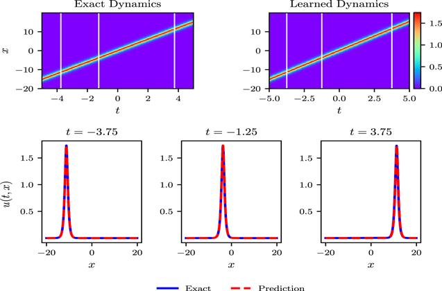
Figure 6. The mKdV equation. Top: a one-soliton solution to the mKdV equation (left panel) is compared to the predicted solution to the learned equation. The model correctly exhibits the dynamics behavior and accurately reproduces the solution with a relative |
3.2. Breather solution
Now, we consider the breather solution, which is not only spatially localized but also time periodic, to the mKdV equation: $ \begin{eqnarray}\left\{\begin{array}{l}{u}_{t}+6{u}^{2}{u}_{x}+{u}_{{xxx}}=0,x\in [-20,20],t\in [-0.3,0.3],\\ u({t}_{0},x)={u}_{0}(x),\\ u(t,-20)=u(t,20)=0.\end{array}\right.\end{eqnarray}$
One could obtain the exact breather solution using some analytical methods [40]:
$ \begin{eqnarray*}\begin{array}{l}u(t,x)=2{\partial }_{x}\left[\arctan \left(\displaystyle \frac{\beta }{\alpha }\displaystyle \frac{\sin (\alpha (x+\delta t))}{\cosh (\beta (x+\gamma t))}\right)\right]\\ \qquad =\ 2\beta {\rm{sech}} (\beta (x+\gamma t))\\ \times \ \left[\displaystyle \frac{\cos (\alpha (x+\delta t))-(\beta /\alpha )\sin (\alpha (x+\delta t))\tanh (\beta (x+\gamma t))}{1+{\left(\beta /\alpha \right)}^{2}{\sin }^{2}(\alpha (x+\delta t)){{\rm{sech}} }^{2}(\beta (x+\gamma t))}\right],\end{array}\end{eqnarray*}$
with$\delta ={\alpha }^{2}-3{\beta }^{2}$ and $\gamma =3{\alpha }^{2}-{\beta }^{2}$ , where α and β are arbitrary constants.
with
When α = 1.5 and β = 1.0, we generate the data of 201 snapshots directly on the regular space–time grid every Δt = 0.003. We generate a smaller training data subset scattered in space and time by randomly sub-sampling N u = 100 initial data and N f = 10 000 collocation points. Specifically, given a set of initial and boundary data, we try to learn the solution u (t, x) by training all learnable parameters of the network. Figure 7 demonstrates the evolution of the breather solution within about a time period (9 ). The top panel of figure 7 compares between the exact dynamics and the predicted solution. The model achieves a relative ${{\mathbb{L}}}_{2}$ error of size 1.05% in a runtime of about 2.2 h. We can see a more detailed assessment in the bottom panel of figure 7 . We present a comparison between the exact solutions and the predicted solutions at different points t = −0.22, 0, 0.23. From figure 7, we observe that the model exactly reproduces the breather pattern.

Figure 7. The mKdV equation. Top: a breather solution to the mKdV equation (left panel) is compared to the predicted solution to the learned equation. The model correctly exhibits the dynamics behavior and accurately reproduces the solution with a relative |
4. The KdV–Burgers equation
The KdV–Burgers equation is often utilized for a large number of nonlinear systems because this model has damping and dispersion terms [41 –43]. Specifically, we consider the KdV–Burgers equation with Dirichlet boundary conditions given by $ \begin{eqnarray}\left\{\begin{array}{l}{u}_{t}+{{uu}}_{x}-\alpha {u}_{{xx}}-\beta {u}_{{xxx}}=0,x\in [-40,40],t\in [-5,5],\\ u({t}_{0},x)={u}_{0}(x),\\ u(t,-40)=u(t,40)=0,\end{array}\right.\end{eqnarray}$ where α and β are constants. In this case, ${ \mathcal N }=-{{uu}}_{x}\,+\alpha {u}_{{xx}}+\beta {u}_{{xxx}}$ .
The exact one-soliton solution, that is actually a kink, is obtained:
$ \begin{eqnarray*}u(t,x)=\displaystyle \frac{3{\alpha }^{2}}{25\beta }\left(2+2\tanh \displaystyle \frac{z}{2}-{{\rm{sech}} }^{2}\displaystyle \frac{z}{2}\right),\end{eqnarray*}$
with$z=\tfrac{\alpha }{5\beta }\left(x-\tfrac{6{\alpha }^{2}}{25\beta }t\right)$ , where α and β are constants.
with
When α = 1.0 and β = −1.0, we generate the data. In this case, we just sample the data on the regular space–time grid every Δt = 0.05 and finally obtain totally 201 snapshots. Out of this data, we generate a smaller training data subset by randomly sub-sampling N u = 100 initial data and N f = 10 000 collocation points. Figure 8 summarizes our result for the kink solution to the KdV–Burgers equation. The top panel of figure 8 compares between the exact dynamics and the predicted spatiotemporal solution and the resulting prediction error is measured at 8.08 × 10⁻³ in the relative ${{\mathbb{L}}}_{2}$ -norm with a runtime of about one and half a minute. More detailed assessments are presented in the middle and bottom panels of figure 8 . Moreover, we present a comparison between the exact solutions and the predicted solutions at different time instants t = −3.75, −1.25, 3.75. This model can accurately capture the kink dynamics behavior of the KdV–Burgers equation.
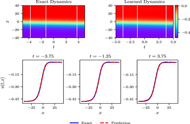
Figure 8. The KdV–Burgers equation. Top: a one-kink solution to the KdVB equation (left panel) is compared to the predicted solution to the learned equation. The model correctly exhibits the dynamics behavior and accurately reproduces the solution with a relative |
5. The STO equation
The STO equation has important applications in many scientific areas. It has been investigated using different analytic methods, such as the Cole–Hopf transformation and Hirota’s bilinear method. Here, we consider the STO equation [44] with the Dirichlet boundary condition given by: $ \begin{eqnarray}\left\{\begin{array}{l}{u}_{t}+3\alpha {u}_{x}^{2}+3\alpha {u}^{2}{u}_{x}+3\alpha {{uu}}_{{xx}}+\alpha {u}_{{xxx}}=0,x\in [-40,40],t\in [-5,5],\\ u({t}_{0},x)={u}_{0}(x),\\ u(t,-40)=a,u(t,40)=b,\end{array}\right.\end{eqnarray}$ where α is an arbitrary constant, and a, b are fixed values which can be easily obtained given an initial condition. In this case, ${ \mathcal N }=-3\alpha {u}_{x}^{2}-3\alpha {u}^{2}{u}_{x}-3\alpha {{uu}}_{{xx}}-\alpha {u}_{{xxx}}$ .
An exact soliton solution is obtained using certain method mentioned above:
$ \begin{eqnarray*}u(t,x)=\displaystyle \frac{{k}_{1}{e}^{{k}_{1}(x-\alpha {k}_{1}^{2}t)}+{k}_{2}{e}^{{k}_{2}(x-\alpha {k}_{2}^{2}t)}}{1+{e}^{{k}_{1}(x-\alpha {k}_{1}^{2}t)}+{e}^{{k}_{2}(x-\alpha {k}_{2}^{2}t)}}.\end{eqnarray*}$
5.1. Soliton fusion
The soliton fusion phenomenon is a resonance-like inelastic interaction where two or more solitons fuse into one single structure or less solitons, that is to say, the total number of solitons is not conserved.
Specifically, when α = 1.0 and k 1 = −1.8, k 2 = 1.0, we obtain the solution data. In this case, we sample the data on the regular space–time grid every Δt = 0.05 and finally obtain totally 201 snapshots. Out of this data, we generate a smaller training data subset by randomly sub-sampling N u = 100 initial-boundary data and N f = 10 000 collocation points. Specifically, given a set of initial and boundary data, we try to learn the solution u (t, x) by tuning all parameters of the network. Figure 9 graphically shows the evolution of the soliton fusion phenomena of the the STO equation (11 ). The top panel of figure 9 compares between the exact dynamics and the predicted spatiotemporal solution. The model achieves a relative ${{\mathbb{L}}}_{2}$ error of size 1.61% in a runtime of approximately 10 minutes. More detailed assessments are presented in the middle and bottom panels of figure 9 . We present a comparison between the exact solutions and the predicted solutions at different time points t = −3.75, −1.25, 3.75.
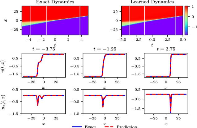
Figure 9. The soliton fusion phenomenon of the STO equation. Top: a solution to the STO equation (left panel) is compared to the predicted solution to the learned equation. The model correctly exhibits the dynamics behavior and accurately reproduces the solution with a relative |
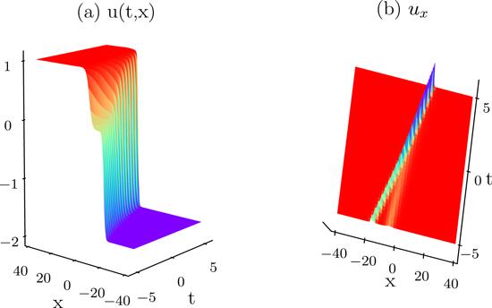
Figure 10. The soliton fusion pattern of the STO equation. (a) The spatiotemporal behavior of the reconstructed solution; (b) the spatiotemporal dynamics of the corresponding potential. |
From figure 4, we can more clearly observe that two solitons with different speeds fuse into a single soliton with a larger amplitude.
5.2. Soliton fission
Now, we consider a sort of inverse of the fusion process, namely, one or several solitons may crack into two or more solitons.
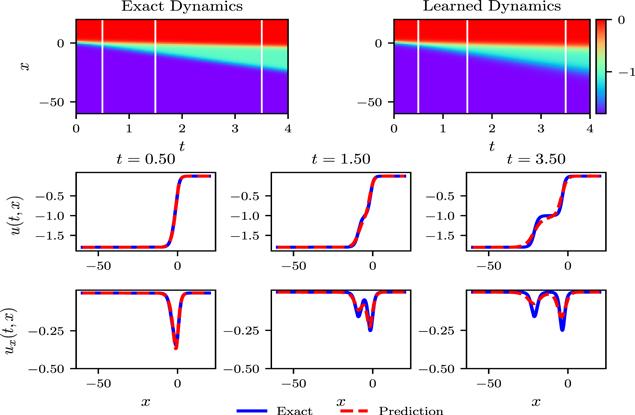
Note that, we reset $x\in [-60,20]$ and $t\in [0,4]$ in this case. When α = −1.0 and k 1 = −1.8, k 2 = −1.0, we obtain the data. In this case, we just sample the data on the regular grid every Δt = 0.008 from t = 0 up to the final instant t = 4 and finally obtain totally 501 snapshots. Out of this data, we generate a smaller training data subset by randomly sub-sampling N u = 200 initial-boundary data and N f = 20 000 collocation points.
For this soliton fission case, the sin(x) activation is often not good, thus we choose the $\tanh (x)$ function as the activation. Specifically, given a set of initial and boundary data, we try to fit the solution u (t, x) by training the network using the loss function (3 ). Figure 11 graphically shows the evolution of the soliton fission process of the the STO equation (11 ). The top panel of figure 11 compares between the exact dynamics and the predicted spatiotemporal solution. The model achieves a relative ${{\mathbb{L}}}_{2}$ error of size 2.41% in a runtime of approximately 11 min. More detailed assessments are presented in the middle and bottom panels of figure 11 . We present a comparison between the exact solutions and the predicted solutions at different points t = 0.5, 1.5, 3.5.
Figure 11. The soliton fission phenomenon of the STO equation. Top: a solution to the STO equation (left panel) is compared to the predicted solution to the learned equation. The model approximately exhibits the dynamics behavior and reproduces the solution with a relative |
This model approximately reconstructs the exact solution from the coarse-grained sampled data. However, from the middle and bottom panels of figure 11, it obviously can not exhibit the vicinity of wave humps well. One could devise more sophisticated sampling strategies to enable adaptive refinement, for instance, by tracking the curvature of the solution. This will be further investigated in the future research.
6. Remarks and discussion
Deep learning offers a quite different approach for modeling these dynamical behaviors by using the training data to parameterize the solution manifold itself; in other words, it learns both the intrinsic features and their interactions from data collected from experiments and simulations. In this paper, we present a neural network framework for extracting soliton dynamics of evolution equations from the spatiotemporal data. The framework provides a universal treatment of (1 + 1)-dimensional third-order nonlinear evolution equations. Specifically, we outline how different categories of soliton solutions (e.g. general soliton solutions, breathers and kinks) to the equations come about due to different choices of initial and boundary data. The results show that the model could recover the different soliton behaviors of these equations fairly well.
Note that a low loss value is a necessary but not sufficient condition for stable training and accurate prediction. For the soliton fission case in the previous section, in particular, the model with low training loss exhibits relatively poor stability and prediction result. In addition, soliton behaviors under certain small perturbations have been studied to some extent [30, 45, 46]. Correspondingly, it is very interesting to extend to the stability of solitons with training the neural network with noisy data. These remain important areas of exploration for future work.