Welcome to visit Communications in Theoretical Physics,
Mathematical Physics

Soliton and other solutions to the (1 + 2)-dimensional chiral nonlinear Schrödinger equation

  • K Hosseini , 1, ,
  • M Mirzazadeh , 2,
Expand
  • 1Department of Mathematics, Rasht Branch, Islamic Azad University, Rasht, Iran
  • 2Department of Engineering Sciences, Faculty of Technology and Engineering, East of Guilan, University of Guilan, P.C. 44891-63157 Rudsar-Vajargah, Iran

Authors to whom any correspondence should be addressed.

Received date: 2020-07-04

  Revised date: 2020-08-10

  Accepted date: 2020-09-10

  Online published: 2020-12-16

Copyright

© 2020 Institute of Theoretical Physics CAS, Chinese Physical Society and IOP Publishing

Abstract

The (1 + 2)-dimensional chiral nonlinear Schrödinger equation (2D-CNLSE) as a nonlinear evolution equation is considered and studied in a detailed manner. To this end, a complex transform is firstly adopted to arrive at the real and imaginary parts of the model, and then, the modified Jacobi elliptic expansion method is formally utilized to derive soliton and other solutions of the 2D-CNLSE. The exact solutions presented in this paper can be classified as topological and nontopological solitons as well as Jacobi elliptic function solutions.

Cite this article

K Hosseini , M Mirzazadeh . Soliton and other solutions to the (1 + 2)-dimensional chiral nonlinear Schrödinger equation[J]. Communications in Theoretical Physics, 2020 , 72(12) : 125008 . DOI: 10.1088/1572-9494/abb87b

1. Introduction

Nishino et al [1] studied a nonlinear evolution equation known as the (1 + 1)-dimensional chiral nonlinear Schrödinger equation (1D-CNLSE) in the form
$\begin{eqnarray*}{\rm{i}}{u}_{t}+{c}_{1}{u}_{xx}+{\rm{i}}{c}_{2}\left(u{u}_{x}^{* }-{u}^{* }{u}_{x}\right)u=0,\end{eqnarray*}$
and obtained its bright and dark solitons. The 1D-CNLSE was established as a one-dimensional reduction of a system describing the edge states of the Fractional Quantum Hall Effect [2]. Thereafter, the (1 + 2)-dimensional form of the chiral nonlinear Schrödinger equation (2D-CNLSE), namely [3-6]
$\begin{eqnarray}\begin{array}{l}{\rm{i}}{u}_{t}+{c}_{1}\left({u}_{xx}+{u}_{yy}\right)+{\rm{i}}\left({c}_{2}\left(u{u}_{x}^{* }-{u}^{* }{u}_{x}\right)\right.\\ \,+\,\left.{c}_{3}\left(u{u}_{y}^{* }-{u}^{* }{u}_{y}\right)\right)u=0,\end{array}\end{eqnarray}$
was studied by a series of researchers using different methods. For example, Biswas [3] obtained chiral solitons of the 2D-CNLSE using several soliton ansatz methods. Eslami [4] used the trial solution method to derive solitons and other solutions of the 2D-CNLSE. Raza and Javid [5] derived exact solutions of the 2D-CNLSE through the modified extended direct algebraic method. Raza and Arshed [6] utilized the sine-Gordon expansion method to obtain chiral bright and dark soliton solutions of the 2D-CNLSE.
It should be mentioned that the first and second terms appeared in equation (1) present the evolution term and the dispersion term, respectively. Besides, ${c}_{2}$ and ${c}_{3}$ signify the coefficients of nonlinear coupling terms. Unfortunately, the 2D-CNLSE is not Galilean invariant and does not possess the Painlevé test [3]. Such features of the 2D-CNLSE reveal the importance of extracting solitons and other solutions to it.
The current paper aims to present soliton and other solutions of the 2D-CNLSE using the modified Jacobi elliptic expansion (MJEE) method [7-14]. To highlight the effectiveness of the MJEE method for handling nonlinear evolution equations, a review of its recent applications is provided below. Ma et al [7] used the MJEE method to construct new exact solutions of MKdV and BBM equations. Hosseini et al [8] obtained solitons and Jacobi elliptic function solutions of the complex Ginzburg-Landau equation using the MJEE method. The reader is referred to [15-36].
The organization of this paper is as follows: in section 2, the MJEE method is described in detail. In section 3, soliton and other solutions of the 2D-CNLSE are constructed using the MJEE method. Finally, conclusions are presented in the last section.

2. The MJEE method

The key ideas of the MJEE method are summarized in this section. To start, consider the following nonlinear ordinary differential equation
$\begin{eqnarray}P\left(u,u^{\prime} ,u^{\prime\prime} ,\,\mathrm{...}\right)=0,^{\prime} =\displaystyle \frac{{\rm{d}}}{{\rm{d}}{\epsilon }}.\end{eqnarray}$
Suppose that the exact solution of equation (2) can be written as a finite series in the form
$\begin{eqnarray}\begin{array}{l}u\left({\epsilon }\right)={a}_{0}+\displaystyle {\sum }_{i=1}^{N}{\left(\displaystyle \frac{J\left({\epsilon }\right)}{1+{J}^{2}\left({\epsilon }\right)}\right)}^{i-1}\left({a}_{i}\displaystyle \frac{J\left({\epsilon }\right)}{1+{J}^{2}\left({\epsilon }\right)}\right.\\ \,\,\,+\,\left.{b}_{i}\displaystyle \frac{1-{J}^{2}\left({\epsilon }\right)}{1+{J}^{2}\left({\epsilon }\right)}\right),\,{a}_{N}\,{\rm{or}}\,{b}_{N}\ne 0,\end{array}\end{eqnarray}$
where ${a}_{0},$ ${a}_{i},$ and ${b}_{i}$ ($1\leqslant i\leqslant N$) are determined later, $N$ is obtained by the balance principle, and $J\left({\epsilon }\right)$ is a Jacobi elliptic function satisfying
$\begin{eqnarray}{\left(J^{\prime} \left({\epsilon }\right)\right)}^{2}=D+E{J}^{2}\left({\epsilon }\right)+F{J}^{4}\left({\epsilon }\right).\end{eqnarray}$
The exact solutions of the Jacobi elliptic equation (4) depending on the parameters $D,$ $E,$ and $F$ have been listed in table 1.
Table 1. Jacobi elliptic function solutions of equation (4).
No. D E F J(ξ)
1 $1$ $-\left({m}^{2}+1\right)$ ${m}^{2}$ ${\rm{sn}}\left(\xi \right)$
2 $1-{m}^{2}$ $2{m}^{2}-1$ $-{m}^{2}$ ${\rm{cn}}\left(\xi \right)$
3 ${m}^{2}$ $-\left({m}^{2}+1\right)$ $1$ ${\rm{ns}}\left(\xi \right)$
4 $-{m}^{2}$ $2{m}^{2}-1$ $1-{m}^{2}$ ${\rm{nc}}\left(\xi \right)$
By inserting the finite series (3) into equation (2) and exerting some operations, we get a nonlinear algebraic system whose solution results in exact solutions of equation (2).
Several useful properties of the Jacobi elliptic functions have been given below:

${{\rm{sn}}}^{2}\left(\xi \right)+{{\rm{cn}}}^{2}\left(\xi \right)=1.$

${\rm{sn}}\left(\xi \right)={\rm{sn}}\left(\xi ,m\right)\to \,\tanh \left(\xi \right)$ when $m\to 1.$

${\rm{ns}}\left(\xi \right)={\left({\rm{sn}}\left(\xi ,m\right)\right)}^{-1}\to \,\coth \left(\xi \right)$ when $m\to 1.$

3. The 2D-CNLSE and its soliton and other solutions

The main aim of this section is to present soliton and other solutions of the 2D-CNLSE using the MJEE method. To this end, a complex transformation is firstly considered as
$\begin{eqnarray}u\left(x,y,t\right)=U\left({\epsilon }\right){{\rm{e}}}^{{\rm{i}}\left({\kappa }_{2}x+{\lambda }_{2}y+{\mu }_{2}t\right)},{\epsilon }={\kappa }_{1}x+{\lambda }_{1}y-{\mu }_{1}t,\end{eqnarray}$
where
${\kappa }_{1}:$ The inverse width of the soliton in the $x$-direction,
${\lambda }_{1}:$ The inverse width of the soliton in the $y$-direction,
${\mu }_{1}:$ The velocity of the soliton,
${\kappa }_{2}:$ The frequency in the $x$-direction,
${\lambda }_{2}:$ The frequency in the $y$-direction,
${\mu }_{2}:$ The soliton frequency.
Considering the complex transformation (5) and the 2D-CNLSE (1) gives
$\begin{eqnarray}\begin{array}{l}{c}_{1}\left({{\kappa }_{1}}^{2}+{{\lambda }_{1}}^{2}\right)\displaystyle \frac{{{\rm{d}}}^{2}U\left({\epsilon }\right)}{{\rm{d}}{{\epsilon }}^{2}}-\left({c}_{1}{{\kappa }_{2}}^{2}+{c}_{1}{{\lambda }_{2}}^{2}+{\mu }_{2}\right)U\left({\epsilon }\right)\\ \,+\,2\left({c}_{2}{\kappa }_{2}+{c}_{3}{\lambda }_{2}\right){U}^{3}\left({\epsilon }\right)=0,\end{array}\end{eqnarray}$
$\begin{eqnarray}\left(2{c}_{1}{\kappa }_{1}{\kappa }_{2}+2{c}_{1}{\lambda }_{1}{\lambda }_{2}-{\mu }_{1}\right)\displaystyle \frac{{\rm{d}}U\left({\epsilon }\right)}{{\rm{d}}{\epsilon }}=0.\end{eqnarray}$
From equation (7), the soliton velocity is found as
$\begin{eqnarray*}{\mu }_{1}=2{c}_{1}\left({\kappa }_{1}{\kappa }_{2}+{\lambda }_{1}{\lambda }_{2}\right).\end{eqnarray*}$
Now, balancing the terms $\tfrac{{{\rm{d}}}^{2}U\left({\epsilon }\right)}{{\rm{d}}{{\epsilon }}^{2}}$ and ${U}^{3}\left({\epsilon }\right)$ appeared in equation (6) results in $N=1.$ Consequently, based on the initial assumption of the MJEE method, the solution of equation (6) can be written as follows
$\begin{eqnarray}U\left({\epsilon }\right)={a}_{0}+{a}_{1}\displaystyle \frac{J\left({\epsilon }\right)}{1+{J}^{2}\left({\epsilon }\right)}+{a}_{2}\displaystyle \frac{1-{J}^{2}\left({\epsilon }\right)}{1+{J}^{2}\left({\epsilon }\right)},\,{a}_{2}={b}_{1},\end{eqnarray}$
where ${a}_{0},$ ${a}_{1},$ and ${a}_{2}$ are unknowns. Substituting the solution (8) into equation (6) and exerting some operations, a system of nonlinear algebraic equations is derived as
$\begin{eqnarray*}\begin{array}{l}-4D{a}_{2}{c}_{1}{{\kappa }_{1}}^{2}-4D{a}_{2}{c}_{1}{{\lambda }_{1}}^{2}+2{{a}_{0}}^{3}{c}_{2}{\kappa }_{2}+2{{a}_{0}}^{3}{c}_{3}{\lambda }_{2}\\ \,+\,6{{a}_{0}}^{2}{a}_{2}{c}_{2}{\kappa }_{2}+6{{a}_{0}}^{2}{a}_{2}{c}_{3}{\lambda }_{2}+6{a}_{0}{{a}_{2}}^{2}{c}_{2}{\kappa }_{2}\\ \,+\,6{a}_{0}{{a}_{2}}^{2}{c}_{3}{\lambda }_{2}+2{{a}_{2}}^{3}{c}_{2}{\kappa }_{2}+2{{a}_{2}}^{3}{c}_{3}{\lambda }_{2}-{a}_{0}{c}_{1}{{\kappa }_{2}}^{2}\\ \,-\,{a}_{0}{c}_{1}{{\lambda }_{2}}^{2}-{a}_{2}{c}_{1}{{\kappa }_{2}}^{2}-{a}_{2}{c}_{1}{{\lambda }_{2}}^{2}-{a}_{0}{\mu }_{2}-{a}_{2}{\mu }_{2}=0,\end{array}\end{eqnarray*}$
$\begin{eqnarray*}\begin{array}{l}-6D{a}_{1}{c}_{1}{{\kappa }_{1}}^{2}-6D{a}_{1}{c}_{1}{{\lambda }_{1}}^{2}+E{a}_{1}{c}_{1}{{\kappa }_{1}}^{2}+E{a}_{1}{c}_{1}{{\lambda }_{1}}^{2}\\ \,+\,6{{a}_{0}}^{2}{a}_{1}{c}_{2}{\kappa }_{2}+6{{a}_{0}}^{2}{a}_{1}{c}_{3}{\lambda }_{2}+12{a}_{0}{a}_{1}{a}_{2}{c}_{2}{\kappa }_{2}\\ \,+\,12{a}_{0}{a}_{1}{a}_{2}{c}_{3}{\lambda }_{2}+6{a}_{1}{{a}_{2}}^{2}{c}_{2}{\kappa }_{2}+6{a}_{1}{{a}_{2}}^{2}{c}_{3}{\lambda }_{2}\\ \,-\,{a}_{1}{c}_{1}{{\kappa }_{2}}^{2}-{a}_{1}{c}_{1}{{\lambda }_{2}}^{2}-{a}_{1}{\mu }_{2}=0,\end{array}\,\end{eqnarray*}$
$\begin{eqnarray*}\begin{array}{l}12D{a}_{2}{c}_{1}{{\kappa }_{1}}^{2}+12D{a}_{2}{c}_{1}{{\lambda }_{1}}^{2}-8E{a}_{2}{c}_{1}{{\kappa }_{1}}^{2}-8E{a}_{2}{c}_{1}{{\lambda }_{1}}^{2}\\ \,+\,6{{a}_{0}}^{3}{c}_{2}{\kappa }_{2}+6{{a}_{0}}^{3}{c}_{3}{\lambda }_{2}+6{{a}_{0}}^{2}{a}_{2}{c}_{2}{\kappa }_{2}+6{{a}_{0}}^{2}{a}_{2}{c}_{3}{\lambda }_{2}\\ \,+\,6{a}_{0}{{a}_{1}}^{2}{c}_{2}{\kappa }_{2}+6{a}_{0}{{a}_{1}}^{2}{c}_{3}{\lambda }_{2}-6{a}_{0}{{a}_{2}}^{2}{c}_{2}{\kappa }_{2}\\ \,-\,6{a}_{0}{{a}_{2}}^{2}{c}_{3}{\lambda }_{2}+6{{a}_{1}}^{2}{a}_{2}{c}_{2}{\kappa }_{2}+6{{a}_{1}}^{2}{a}_{2}{c}_{3}{\lambda }_{2}\\ \,-\,6{{a}_{2}}^{3}{c}_{2}{\kappa }_{2}-6{{a}_{2}}^{3}{c}_{3}{\lambda }_{2}-3{a}_{0}{c}_{1}{{\kappa }_{2}}^{2}-3{a}_{0}{c}_{1}{{\lambda }_{2}}^{2}\\ \,-\,{a}_{2}{c}_{1}{{\kappa }_{2}}^{2}-{a}_{2}{c}_{1}{{\lambda }_{2}}^{2}-3{a}_{0}{\mu }_{2}-{a}_{2}{\mu }_{2}=0,\end{array}\end{eqnarray*}$
$\begin{eqnarray*}\begin{array}{l}2D{a}_{1}{c}_{1}{{\kappa }_{1}}^{2}+2D{a}_{1}{c}_{1}{{\lambda }_{1}}^{2}-6E{a}_{1}{c}_{1}{{\kappa }_{1}}^{2}-6E{a}_{1}{c}_{1}{{\lambda }_{1}}^{2}\\ \,+\,2F{a}_{1}{c}_{1}{{\kappa }_{1}}^{2}+2F{a}_{1}{c}_{1}{{\lambda }_{1}}^{2}+12{{a}_{0}}^{2}{a}_{1}{c}_{2}{\kappa }_{2}\\ \,+\,12{{a}_{0}}^{2}{a}_{1}{c}_{3}{\lambda }_{2}+2{{a}_{1}}^{3}{c}_{2}{\kappa }_{2}+2{{a}_{1}}^{3}{c}_{3}{\lambda }_{2}-12{a}_{1}{{a}_{2}}^{2}{c}_{2}{\kappa }_{2}\\ \,-\,12{a}_{1}{{a}_{2}}^{2}{c}_{3}{\lambda }_{2}-2{a}_{1}{c}_{1}{{\kappa }_{2}}^{2}-2{a}_{1}{c}_{1}{{\lambda }_{2}}^{2}-2{a}_{1}{\mu }_{2}=0,\end{array}\end{eqnarray*}$
$\begin{eqnarray*}\begin{array}{l}8E{a}_{2}{c}_{1}{{\kappa }_{1}}^{2}+8E{a}_{2}{c}_{1}{{\lambda }_{1}}^{2}-12F{a}_{2}{c}_{1}{{\kappa }_{1}}^{2}-12F{a}_{2}{c}_{1}{{\lambda }_{1}}^{2}\\ \,+\,6{{a}_{0}}^{3}{c}_{2}{\kappa }_{2}+6{{a}_{0}}^{3}{c}_{3}{\lambda }_{2}-6{{a}_{0}}^{2}{a}_{2}{c}_{2}{\kappa }_{2}-6{{a}_{0}}^{2}{a}_{2}{c}_{3}{\lambda }_{2}\\ \,+\,6{a}_{0}{{a}_{1}}^{2}{c}_{2}{\kappa }_{2}+6{a}_{0}{{a}_{1}}^{2}{c}_{3}{\lambda }_{2}-6{a}_{0}{{a}_{2}}^{2}{c}_{2}{\kappa }_{2}\\ \,-\,6{a}_{0}{{a}_{2}}^{2}{c}_{3}{\lambda }_{2}-6{{a}_{1}}^{2}{a}_{2}{c}_{2}{\kappa }_{2}-6{{a}_{1}}^{2}{a}_{2}{c}_{3}{\lambda }_{2}\\ \,+\,6{{a}_{2}}^{3}{c}_{2}{\kappa }_{2}+6{{a}_{2}}^{3}{c}_{3}{\lambda }_{2}-3{a}_{0}{c}_{1}{{\kappa }_{2}}^{2}-3{a}_{0}{c}_{1}{{\lambda }_{2}}^{2}\\ \,+\,{a}_{2}{c}_{1}{{\kappa }_{2}}^{2}+{a}_{2}{c}_{1}{{\lambda }_{2}}^{2}-3{a}_{0}{\mu }_{2}+{a}_{2}{\mu }_{2}=0,\end{array}\end{eqnarray*}$
$\begin{eqnarray*}\begin{array}{l}E{a}_{1}{c}_{1}{{\kappa }_{1}}^{2}+E{a}_{1}{c}_{1}{{\lambda }_{1}}^{2}-6F{a}_{1}{c}_{1}{{\kappa }_{1}}^{2}-6F{a}_{1}{c}_{1}{{\lambda }_{1}}^{2}\\ \,+\,6{{a}_{0}}^{2}{a}_{1}{c}_{2}{\kappa }_{2}+6{{a}_{0}}^{2}{a}_{1}{c}_{3}{\lambda }_{2}-12{a}_{0}{a}_{1}{a}_{2}{c}_{2}{\kappa }_{2}\\ \,-\,12{a}_{0}{a}_{1}{a}_{2}{c}_{3}{\lambda }_{2}+6{a}_{1}{{a}_{2}}^{2}{c}_{2}{\kappa }_{2}+6{a}_{1}{{a}_{2}}^{2}{c}_{3}{\lambda }_{2}\\ \,-\,{a}_{1}{c}_{1}{{\kappa }_{2}}^{2}-{a}_{1}{c}_{1}{{\lambda }_{2}}^{2}-{a}_{1}{\mu }_{2}=0,\end{array}\,\end{eqnarray*}$
$\begin{eqnarray*}\begin{array}{l}4F{a}_{2}{c}_{1}{{\kappa }_{1}}^{2}+4F{a}_{2}{c}_{1}{{\lambda }_{1}}^{2}+2{{a}_{0}}^{3}{c}_{2}{\kappa }_{2}+2{{a}_{0}}^{3}{c}_{3}{\lambda }_{2}\\ \,-\,6{{a}_{0}}^{2}{a}_{2}{c}_{2}{\kappa }_{2}-6{{a}_{0}}^{2}{a}_{2}{c}_{3}{\lambda }_{2}+6{a}_{0}{{a}_{2}}^{2}{c}_{2}{\kappa }_{2}\\ \,+\,6{a}_{0}{{a}_{2}}^{2}{c}_{3}{\lambda }_{2}-2{{a}_{2}}^{3}{c}_{2}{\kappa }_{2}-2{{a}_{2}}^{3}{c}_{3}{\lambda }_{2}-{a}_{0}{c}_{1}{{\kappa }_{2}}^{2}\\ \,-\,{a}_{0}{c}_{1}{{\lambda }_{2}}^{2}+{a}_{2}{c}_{1}{{\kappa }_{2}}^{2}+{a}_{2}{c}_{1}{{\lambda }_{2}}^{2}-{a}_{0}{\mu }_{2}+{a}_{2}{\mu }_{2}=0,\end{array}\end{eqnarray*}$
whose solution leads to the following cases:

When $D=1,$ $E=-\left({m}^{2}+1\right),$ and $F={m}^{2},$ one derives

$\begin{eqnarray*}\begin{array}{l}\bullet \,{a}_{0}=0,{a}_{1}=\pm 4\sqrt{-\displaystyle \frac{{c}_{1}{{\kappa }_{1}}^{2}+{c}_{1}{{\lambda }_{1}}^{2}}{{c}_{2}{\kappa }_{2}+{c}_{3}{\lambda }_{2}}},{a}_{2}=0,\\ \,\,{\mu }_{2}=-\left(8{{\kappa }_{1}}^{2}+{{\kappa }_{2}}^{2}+8{{\lambda }_{1}}^{2}+{{\lambda }_{2}}^{2}\right){c}_{1},m=1,\end{array}\,\end{eqnarray*}$
$\begin{eqnarray*}\begin{array}{l}\bullet \,{a}_{0}=0,{a}_{1}=0,{a}_{2}=\pm 2\sqrt{-\displaystyle \frac{-{c}_{1}{{\kappa }_{1}}^{2}-{c}_{1}{{\lambda }_{1}}^{2}}{{c}_{2}{\kappa }_{2}+{c}_{3}{\lambda }_{2}}},\\ \,\,{\mu }_{2}=\left(4{{\kappa }_{1}}^{2}-{{\kappa }_{2}}^{2}+4{{\lambda }_{1}}^{2}-{{\lambda }_{2}}^{2}\right){c}_{1},m=1,\end{array}\end{eqnarray*}$
$\begin{eqnarray*}\begin{array}{l}\bullet \,{a}_{0}=0,{a}_{1}=2\sqrt{-\displaystyle \frac{{c}_{1}{{\kappa }_{1}}^{2}+{c}_{1}{{\lambda }_{1}}^{2}}{{c}_{2}{\kappa }_{2}+{c}_{3}{\lambda }_{2}}},\\ \,\,{a}_{2}=\pm \,\sqrt{-\displaystyle \frac{-{c}_{1}{{\kappa }_{1}}^{2}-{c}_{1}{{\lambda }_{1}}^{2}}{{c}_{2}{\kappa }_{2}+{c}_{3}{\lambda }_{2}}},\\ \,\,{\mu }_{2}=-\left(2{{\kappa }_{1}}^{2}+{{\kappa }_{2}}^{2}+2{{\lambda }_{1}}^{2}+{{\lambda }_{2}}^{2}\right){c}_{1},m=1.\end{array}\end{eqnarray*}$
Now, the exact solutions of the 2D-CNLSE can be constructed as follows
$\begin{eqnarray*}\begin{array}{l}{u}_{1,2}\left(x,y,t\right)=\pm 4\sqrt{-\displaystyle \frac{{c}_{1}{{\kappa }_{1}}^{2}+{c}_{1}{{\lambda }_{1}}^{2}}{{c}_{2}{\kappa }_{2}+{c}_{3}{\lambda }_{2}}}\\ \,\times \,\displaystyle \frac{\tanh \left({\kappa }_{1}x+{\lambda }_{1}y-2{c}_{1}\left({\kappa }_{1}{\kappa }_{2}+{\lambda }_{1}{\lambda }_{2}\right)t\right)}{1+{\tanh }^{2}\left({\kappa }_{1}x+{\lambda }_{1}y-2{c}_{1}\left({\kappa }_{1}{\kappa }_{2}+{\lambda }_{1}{\lambda }_{2}\right)t\right)}\\ \,\times \,{{\rm{e}}}^{{\rm{i}}\left({\kappa }_{2}x+{\lambda }_{2}y-\left(8{{\kappa }_{1}}^{2}+{{\kappa }_{2}}^{2}+8{{\lambda }_{1}}^{2}+{{\lambda }_{2}}^{2}\right){c}_{1}t\right)},\end{array}\end{eqnarray*}$
$\begin{eqnarray*}\begin{array}{l}{u}_{3,4}\left(x,y,t\right)=\pm 2\sqrt{-\displaystyle \frac{-{c}_{1}{{\kappa }_{1}}^{2}-{c}_{1}{{\lambda }_{1}}^{2}}{{c}_{2}{\kappa }_{2}+{c}_{3}{\lambda }_{2}}}\\ \,\times \,\displaystyle \frac{1-{\tanh }^{2}\left({\kappa }_{1}x+{\lambda }_{1}y-2{c}_{1}\left({\kappa }_{1}{\kappa }_{2}+{\lambda }_{1}{\lambda }_{2}\right)t\right)}{1+{\tanh }^{2}\left({\kappa }_{1}x+{\lambda }_{1}y-2{c}_{1}\left({\kappa }_{1}{\kappa }_{2}+{\lambda }_{1}{\lambda }_{2}\right)t\right)}\\ \,\times \,{{\rm{e}}}^{{\rm{i}}\left({\kappa }_{2}x+{\lambda }_{2}y+\left(4{{\kappa }_{1}}^{2}-{{\kappa }_{2}}^{2}+4{{\lambda }_{1}}^{2}-{{\lambda }_{2}}^{2}\right){c}_{1}t\right)},\end{array}\end{eqnarray*}$
$\begin{eqnarray*}\begin{array}{l}{u}_{5,6}\left(x,y,t\right)=\left(2\sqrt{-\displaystyle \frac{{c}_{1}{{\kappa }_{1}}^{2}+{c}_{1}{{\lambda }_{1}}^{2}}{{c}_{2}{\kappa }_{2}+{c}_{3}{\lambda }_{2}}}\right.\\ \,\times \,\displaystyle \frac{\tanh \left({\kappa }_{1}x+{\lambda }_{1}y-2{c}_{1}\left({\kappa }_{1}{\kappa }_{2}+{\lambda }_{1}{\lambda }_{2}\right)t\right)}{1+{\tanh }^{2}\left({\kappa }_{1}x+{\lambda }_{1}y-2{c}_{1}\left({\kappa }_{1}{\kappa }_{2}+{\lambda }_{1}{\lambda }_{2}\right)t\right)}\\ \,\pm \,\sqrt{-\displaystyle \frac{-{c}_{1}{{\kappa }_{1}}^{2}-{c}_{1}{{\lambda }_{1}}^{2}}{{c}_{2}{\kappa }_{2}+{c}_{3}{\lambda }_{2}}}\\ \left.\,\times \,\displaystyle \frac{1-{\tanh }^{2}\left({\kappa }_{1}x+{\lambda }_{1}y-2{c}_{1}\left({\kappa }_{1}{\kappa }_{2}+{\lambda }_{1}{\lambda }_{2}\right)t\right)}{1+{\tanh }^{2}\left({\kappa }_{1}x+{\lambda }_{1}y-2{c}_{1}\left({\kappa }_{1}{\kappa }_{2}+{\lambda }_{1}{\lambda }_{2}\right)t\right)}\right)\\ \,\times \,{{\rm{e}}}^{{\rm{i}}\left({\kappa }_{2}x+{\lambda }_{2}y-\left(2{{\kappa }_{1}}^{2}+{{\kappa }_{2}}^{2}+2{{\lambda }_{1}}^{2}+{{\lambda }_{2}}^{2}\right){c}_{1}t\right)}.\end{array}\end{eqnarray*}$

When $D=1-{m}^{2},$ $E=2{m}^{2}-1,$ and $F=-{m}^{2},$ one obtains

$\begin{eqnarray*}\begin{array}{l}{a}_{0}=\pm \sqrt{-\displaystyle \frac{-{c}_{1}{{\kappa }_{1}}^{2}-{c}_{1}{{\lambda }_{1}}^{2}}{4{c}_{2}{\kappa }_{2}+4{c}_{3}{\lambda }_{2}}},{a}_{1}=0,\\ {a}_{2}=\pm \displaystyle \frac{1}{2}\displaystyle \frac{{c}_{1}\left({{\kappa }_{1}}^{2}+{{\lambda }_{1}}^{2}\right)}{{c}_{2}{\kappa }_{2}+{c}_{3}{\lambda }_{2}}\displaystyle \frac{1}{\sqrt{-\tfrac{-{c}_{1}{{\kappa }_{1}}^{2}-{c}_{1}{{\lambda }_{1}}^{2}}{4{c}_{2}{\kappa }_{2}+4{c}_{3}{\lambda }_{2}}}},\\ {\mu }_{2}=\displaystyle \frac{1}{2}\left(5{{\kappa }_{1}}^{2}-2{{\kappa }_{2}}^{2}+5{{\lambda }_{1}}^{2}-2{{\lambda }_{2}}^{2}\right){c}_{1},\,m=\displaystyle \frac{1}{2}.\end{array}\end{eqnarray*}$
Now, the exact solutions of the 2D-CNLSE can be established as follows
$\begin{eqnarray*}\begin{array}{l}{u}_{7,8}\left(x,y,t\right)=\pm \sqrt{-\displaystyle \frac{-{c}_{1}{{\kappa }_{1}}^{2}-{c}_{1}{{\lambda }_{1}}^{2}}{4{c}_{2}{\kappa }_{2}+4{c}_{3}{\lambda }_{2}}}\pm \displaystyle \frac{1}{2}\displaystyle \frac{{c}_{1}\left({{\kappa }_{1}}^{2}+{{\lambda }_{1}}^{2}\right)}{{c}_{2}{\kappa }_{2}+{c}_{3}{\lambda }_{2}}\\ \,\times \,\displaystyle \frac{1}{\sqrt{-\tfrac{-{c}_{1}{{\kappa }_{1}}^{2}-{c}_{1}{{\lambda }_{1}}^{2}}{4{c}_{2}{\kappa }_{2}+4{c}_{3}{\lambda }_{2}}}}\\ \,\times \,\displaystyle \frac{1-{{\rm{cn}}}^{2}\left({\kappa }_{1}x+{\lambda }_{1}y-2{c}_{1}\left({\kappa }_{1}{\kappa }_{2}+{\lambda }_{1}{\lambda }_{2}\right)t,\tfrac{1}{2}\right)}{1+{{\rm{cn}}}^{2}\left({\kappa }_{1}x+{\lambda }_{1}y-2{c}_{1}\left({\kappa }_{1}{\kappa }_{2}+{\lambda }_{1}{\lambda }_{2}\right)t,\tfrac{1}{2}\right)}\\ \,\times \,{{\rm{e}}}^{{\rm{i}}\left({\kappa }_{2}x+{\lambda }_{2}y+\displaystyle \frac{1}{2}\left(5{{\kappa }_{1}}^{2}-2{{\kappa }_{2}}^{2}+5{{\lambda }_{1}}^{2}-2{{\lambda }_{2}}^{2}\right){c}_{1}t\right)}.\end{array}\end{eqnarray*}$

When $D={m}^{2},$ $E=-\left({m}^{2}+1\right),$ and $F=1,$ one derives

$\begin{eqnarray*}\begin{array}{l}\bullet \,{a}_{0}=0,\,{a}_{1}=\pm 4\sqrt{-\displaystyle \frac{{c}_{1}{{\kappa }_{1}}^{2}+{c}_{1}{{\lambda }_{1}}^{2}}{{c}_{2}{\kappa }_{2}+{c}_{3}{\lambda }_{2}}},\,{a}_{2}=0,\\ \,\,{\mu }_{2}=-\left(8{{\kappa }_{1}}^{2}+{{\kappa }_{2}}^{2}+8{{\lambda }_{1}}^{2}+{{\lambda }_{2}}^{2}\right){c}_{1},\,m=1,\end{array}\,\end{eqnarray*}$
$\begin{eqnarray*}\begin{array}{l}\bullet \,{a}_{0}=0,\,{a}_{1}=0,\,{a}_{2}=\pm 2\sqrt{-\displaystyle \frac{-{c}_{1}{{\kappa }_{1}}^{2}-{c}_{1}{{\lambda }_{1}}^{2}}{{c}_{2}{\kappa }_{2}+{c}_{3}{\lambda }_{2}}},\\ \,\,{\mu }_{2}=\left(4{{\kappa }_{1}}^{2}-{{\kappa }_{2}}^{2}+4{{\lambda }_{1}}^{2}-{{\lambda }_{2}}^{2}\right){c}_{1},\,m=1,\end{array}\end{eqnarray*}$
$\begin{eqnarray*}\begin{array}{l}\bullet \,{a}_{0}=0,{a}_{1}=2\sqrt{-\displaystyle \frac{{c}_{1}{{\kappa }_{1}}^{2}+{c}_{1}{{\lambda }_{1}}^{2}}{{c}_{2}{\kappa }_{2}+{c}_{3}{\lambda }_{2}}},\\ \,\,{a}_{2}=\pm \sqrt{-\displaystyle \frac{-{c}_{1}{{\kappa }_{1}}^{2}-{c}_{1}{{\lambda }_{1}}^{2}}{{c}_{2}{\kappa }_{2}+{c}_{3}{\lambda }_{2}}},\\ \,\,{\mu }_{2}=-\left(2{{\kappa }_{1}}^{2}+{{\kappa }_{2}}^{2}+2{{\lambda }_{1}}^{2}+{{\lambda }_{2}}^{2}\right){c}_{1},m=1.\end{array}\end{eqnarray*}$
Now, the exact solutions of the 2D-CNLSE can be constructed as follows
$\begin{eqnarray*}\begin{array}{l}{u}_{9,10}\left(x,y,t\right)=\pm 4\sqrt{-\displaystyle \frac{{c}_{1}{{\kappa }_{1}}^{2}+{c}_{1}{{\lambda }_{1}}^{2}}{{c}_{2}{\kappa }_{2}+{c}_{3}{\lambda }_{2}}}\\ \,\times \,\displaystyle \frac{\coth \left({\kappa }_{1}x+{\lambda }_{1}y-2{c}_{1}\left({\kappa }_{1}{\kappa }_{2}+{\lambda }_{1}{\lambda }_{2}\right)t\right)}{1+{\coth }^{2}\left({\kappa }_{1}x+{\lambda }_{1}y-2{c}_{1}\left({\kappa }_{1}{\kappa }_{2}+{\lambda }_{1}{\lambda }_{2}\right)t\right)}\\ \,\times \,{{\rm{e}}}^{{\rm{i}}\left({\kappa }_{2}x+{\lambda }_{2}y-\left(8{{\kappa }_{1}}^{2}+{{\kappa }_{2}}^{2}+8{{\lambda }_{1}}^{2}+{{\lambda }_{2}}^{2}\right){c}_{1}t\right)},\end{array}\end{eqnarray*}$
$\begin{eqnarray*}\begin{array}{l}{u}_{11,12}\left(x,y,t\right)=\pm 2\sqrt{-\displaystyle \frac{-{c}_{1}{{\kappa }_{1}}^{2}-{c}_{1}{{\lambda }_{1}}^{2}}{{c}_{2}{\kappa }_{2}+{c}_{3}{\lambda }_{2}}}\\ \,\times \,\displaystyle \frac{1-{\coth }^{2}\left({\kappa }_{1}x+{\lambda }_{1}y-2{c}_{1}\left({\kappa }_{1}{\kappa }_{2}+{\lambda }_{1}{\lambda }_{2}\right)t\right)}{1+{\coth }^{2}\left({\kappa }_{1}x+{\lambda }_{1}y-2{c}_{1}\left({\kappa }_{1}{\kappa }_{2}+{\lambda }_{1}{\lambda }_{2}\right)t\right)}\\ \,\times \,{{\rm{e}}}^{{\rm{i}}\left({\kappa }_{2}x+{\lambda }_{2}y+\left(4{{\kappa }_{1}}^{2}-{{\kappa }_{2}}^{2}+4{{\lambda }_{1}}^{2}-{{\lambda }_{2}}^{2}\right){c}_{1}t\right)},\end{array}\end{eqnarray*}$
$\begin{eqnarray*}\begin{array}{l}{u}_{13,14}\left(x,y,t\right)=\left(2\sqrt{-\displaystyle \frac{{c}_{1}{{\kappa }_{1}}^{2}+{c}_{1}{{\lambda }_{1}}^{2}}{{c}_{2}{\kappa }_{2}+{c}_{3}{\lambda }_{2}}}\right.\\ \,\times \,\displaystyle \frac{\coth \left({\kappa }_{1}x+{\lambda }_{1}y-2{c}_{1}\left({\kappa }_{1}{\kappa }_{2}+{\lambda }_{1}{\lambda }_{2}\right)t\right)}{1+{\coth }^{2}\left({\kappa }_{1}x+{\lambda }_{1}y-2{c}_{1}\left({\kappa }_{1}{\kappa }_{2}+{\lambda }_{1}{\lambda }_{2}\right)t\right)}\\ \,\pm \,\sqrt{-\displaystyle \frac{-{c}_{1}{{\kappa }_{1}}^{2}-{c}_{1}{{\lambda }_{1}}^{2}}{{c}_{2}{\kappa }_{2}+{c}_{3}{\lambda }_{2}}}\\ \,\times \,\displaystyle \frac{1-{\coth }^{2}\left({\kappa }_{1}x+{\lambda }_{1}y-2{c}_{1}\left({\kappa }_{1}{\kappa }_{2}+{\lambda }_{1}{\lambda }_{2}\right)t\right)}{1+{\coth }^{2}\left({\kappa }_{1}x+{\lambda }_{1}y-2{c}_{1}\left({\kappa }_{1}{\kappa }_{2}+{\lambda }_{1}{\lambda }_{2}\right)t\right)}\\ \,\times \,{{\rm{e}}}^{{\rm{i}}\left({\kappa }_{2}x+{\lambda }_{2}y-\left(2{{\kappa }_{1}}^{2}+{{\kappa }_{2}}^{2}+2{{\lambda }_{1}}^{2}+{{\lambda }_{2}}^{2}\right){c}_{1}t\right)}.\end{array}\end{eqnarray*}$

When $D=-{m}^{2},$ $E=2{m}^{2}-1,$ and $F=1-{m}^{2},$ one obtains

$\begin{eqnarray*}\begin{array}{l}{a}_{0}=\pm \sqrt{-\displaystyle \frac{-{c}_{1}{{\kappa }_{1}}^{2}-{c}_{1}{{\lambda }_{1}}^{2}}{4{c}_{2}{\kappa }_{2}+4{c}_{3}{\lambda }_{2}}},{a}_{1}=0,\\ {a}_{2}=\mp \displaystyle \frac{1}{2}\displaystyle \frac{{c}_{1}\left({{\kappa }_{1}}^{2}+{{\lambda }_{1}}^{2}\right)}{{c}_{2}{\kappa }_{2}+{c}_{3}{\lambda }_{2}}\displaystyle \frac{1}{\sqrt{-\tfrac{-{c}_{1}{{\kappa }_{1}}^{2}-{c}_{1}{{\lambda }_{1}}^{2}}{4{c}_{2}{\kappa }_{2}+4{c}_{3}{\lambda }_{2}}}},\\ {\mu }_{2}=\displaystyle \frac{1}{2}\left(5{{\kappa }_{1}}^{2}-2{{\kappa }_{2}}^{2}+5{{\lambda }_{1}}^{2}-2{{\lambda }_{2}}^{2}\right){c}_{1},m=\displaystyle \frac{1}{2}.\end{array}\end{eqnarray*}$
Now, the exact solutions of the 2D-CNLSE can be established as follows
$\begin{eqnarray*}\begin{array}{l}{u}_{15,16}\left(x,y,t\right)=\pm \sqrt{-\displaystyle \frac{-{c}_{1}{{\kappa }_{1}}^{2}-{c}_{1}{{\lambda }_{1}}^{2}}{4{c}_{2}{\kappa }_{2}+4{c}_{3}{\lambda }_{2}}}\mp \displaystyle \frac{1}{2}\displaystyle \frac{{c}_{1}\left({{\kappa }_{1}}^{2}+{{\lambda }_{1}}^{2}\right)}{{c}_{2}{\kappa }_{2}+{c}_{3}{\lambda }_{2}}\\ \,\times \,\displaystyle \frac{1}{\sqrt{-\tfrac{-{c}_{1}{{\kappa }_{1}}^{2}-{c}_{1}{{\lambda }_{1}}^{2}}{4{c}_{2}{\kappa }_{2}+4{c}_{3}{\lambda }_{2}}}}\\ \,\times \,\displaystyle \frac{1-{{\rm{nc}}}^{2}\left({\kappa }_{1}x+{\lambda }_{1}y-2{c}_{1}\left({\kappa }_{1}{\kappa }_{2}+{\lambda }_{1}{\lambda }_{2}\right)t,\tfrac{1}{2}\right)}{1+{{\rm{nc}}}^{2}\left({\kappa }_{1}x+{\lambda }_{1}y-2{c}_{1}\left({\kappa }_{1}{\kappa }_{2}+{\lambda }_{1}{\lambda }_{2}\right)t,\tfrac{1}{2}\right)}\\ \,\times \,{{\rm{e}}}^{{\rm{i}}\left({\kappa }_{2}x+{\lambda }_{2}y+\displaystyle \frac{1}{2}\left(5{{\kappa }_{1}}^{2}-2{{\kappa }_{2}}^{2}+5{{\lambda }_{1}}^{2}-2{{\lambda }_{2}}^{2}\right){c}_{1}t\right)}.\end{array}\end{eqnarray*}$
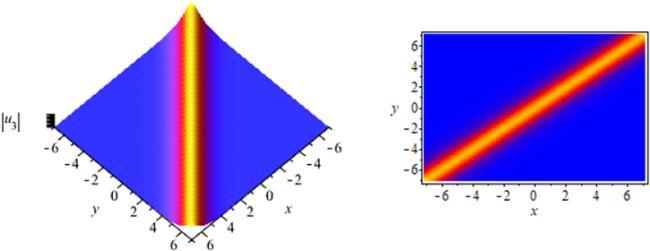
Figures 1 and 2 present the 3-dimensional and density plots of $\left|{u}_{1}\left(x,y,t\right)\right|$ and $\left|{u}_{3}\left(x,y,t\right)\right|$ for a series of suitable parameters. More precisely, the parameters ${c}_{1}=-0.1,$ ${c}_{2}=0.1,$ ${c}_{3}=0.1,$ ${\kappa }_{1}=0.3,$ ${\kappa }_{2}=0.3,$ ${\lambda }_{1}=-0.3,$ and ${\lambda }_{2}=0.3$ have been used to portray figure 1 while the parameters ${c}_{1}=0.1,$ ${c}_{2}=0.1,$ ${c}_{3}=0.1,$ ${\kappa }_{1}=0.7,$ ${\kappa }_{2}=0.7,$ ${\lambda }_{1}=-0.7,$ and ${\lambda }_{2}=0.7$ have been utilized to depict figure 2. Clearly, figure 1 shows a dark or topological soliton while figure 2 indicates a bright or nontopological soliton.

According to the knowledge of the authors, the results given in the current paper are new and have not been presented previously.

The results presented in the current research work were examined by Maple, confirming their correctness.

Figure 1. The 3-dimensional and density plots of $\left|{u}_{1}\left(x,y,t\right)\right|$ for ${c}_{1}=-0.1,$ ${c}_{2}=0.1,$ ${c}_{3}=0.1,$ ${\kappa }_{1}=0.3,$ ${\kappa }_{2}=0.3,$ ${\lambda }_{1}=-0.3,$ ${\lambda }_{2}=0.3,$ and $t=0.$
Figure 2. The 3-dimensional and density plots of $\left|{u}_{3}\left(x,y,t\right)\right|$ for ${c}_{1}=0.1,$ ${c}_{2}=0.1,$ ${c}_{3}=0.1,$ ${\kappa }_{1}=0.7,$ ${\kappa }_{2}=0.7,$ ${\lambda }_{1}=-0.7,$ ${\lambda }_{2}=0.7,$ and $t=0.$

4. Conclusion

The main aim of the current article was to study a nonlinear evolution equation referred to as the 2D-CNLSE in mathematical physics. The study firstly progressed with adopting a complex transform to reduce the 2D-CNLSE to a nonlinear ODE in the real domain with a known soliton velocity. The MJEE method was then adopted to obtain soliton and other solutions of the 2D-CNLSE that were classified as topological and nontopological solitons as well as Jacobi elliptic function solutions. The present article provided useful information regarding the 2D-CNLSE and its exact solutions.
1
Nishino A Umeno Y Wadati M 1998 Chiral nonlinear Schrödinger equation Chaos, Solitons Fractals 9 1063 1069

DOI

2
Aglietti U Griguolo L Jackiw R Pi S Y Semirara D 1996 Anyons and chiral solitons on a line Phys. Rev. Lett. 77 4406 4409

DOI

3
Biswas A 2009 Chiral solitons in 1 + 2 dimensions Int. J. Theor. Phys. 48 3403 3409

DOI

4
Eslami M 2016 Trial solution technique to chiral nonlinear Schrodinger's equation in (1 + 2)-dimensions Nonlinear Dyn. 85 813 816

DOI

5
Raza N Javid A 2019 Optical dark and dark-singular soliton solutions of (1 + 2)-dimensional chiral nonlinear Schrodinger's equation Waves Random Complex Media 29 496 508

DOI

6
Raza N Arshed S 2020 Chiral bright and dark soliton solutions of Schrödinger's equation in (1 + 2)-dimensions Ain Shams Eng. J.

DOI

7
Ma H C Zhang Z P Deng A P 2012 A new periodic solution to Jacobi elliptic functions of MKdV equation and BBM equation Acta Math. Appl. Sin. 28 409 415

DOI

8
Hosseini K Mirzazadeh M Osman M S Al Qurashi M Baleanu D 2020 Solitons and Jacobi elliptic function solutions to the complex Ginzburg-Landau equation Front. Phys. 8 225

DOI

9
Zayed E M E Shohib R M A Biswas A Yıldırım Y Mallawi F Belic M R 2019 Chirped and chirp-free solitons in optical fiber Bragg gratings with dispersive reflectivity having parabolic law nonlinearity by Jacobi's elliptic function Results Phys. 15 102784

DOI

10
Zayed E M E Alngar M E M 2020 Optical solitons in birefringent fibers with Biswas-Arshed model by generalized Jacobi elliptic function expansion method Optik 203 163922

DOI

11
Hosseini K Mirzazadeh M Ilie M Gómez-Aguilar J F 2020 Biswas-Arshed equation with the beta time derivative: optical solitons and other solutions Optik 217 164801

DOI

12
El-Sheikh M M A Seadawy A R Ahmed H M Arnous A H Rabie W B 2020 Dispersive and propagation of shallow water waves as a higher order nonlinear Boussinesq-like dynamical wave equations Physica A 537 122662

DOI

13
Hosseini K Mirzazadeh M Vahidi J Asghari R 2020 Optical wave structures to the Fokas-Lenells equation Optik 207 164450

DOI

14
Hosseini K Matinfar M Mirzazadeh M 2020 A (3 + 1)-dimensional resonant nonlinear Schrödinger equation and its Jacobi elliptic and exponential function solutions Optik 207 164458

DOI

15
Hosseini K Mirzazadeh M Ilie M Radmehr S 2020 Dynamics of optical solitons in the perturbed Gerdjikov-Ivanov equation Optik 206 164350

DOI

16
Hosseini K Osman M S Mirzazadeh M Rabiei F 2020 Investigation of different wave structures to the generalized third-order nonlinear Scrödinger equation Optik 206 164259

DOI

17
Hosseini K Mirzazadeh M Zhou Q Liu Y Moradi M 2019 Analytic study on chirped optical solitons in nonlinear metamaterials with higher order effects Laser Phys. 29 095402

DOI

18
Hosseini K Mirzazadeh M Rabiei F Baskonus H M Yel G 2020 Dark optical solitons to the Biswas-Arshed equation with high order dispersions and absence of self-phase modulation Optik 209 164576

DOI

19
Hosseini K Ma W X Ansari R Mirzazadeh M Pouyanmehr R Samadani F 2020 Evolutionary behavior of rational wave solutions to the (4 + 1)-dimensional Boiti-Leon-Manna-Pempinelli equation Phys. Scr. 95 065208

DOI

20
Biswas A Arshed S 2018 Optical solitons in presence of higher order dispersions and absence of self-phase modulation Optik 174 452 459

DOI

21
Biswas A Ullah M Z Zhou Q Moshokoa S P Triki H Belic M 2017 Resonant optical solitons with quadratic-cubic nonlinearity by semi-inverse variational principle Optik 145 18 21

DOI

22
Kumar S Malik S Biswas A Yıldırım Y Alshomrani A S Belic M R 2020 Optical solitons with generalized anti-cubic nonlinearity by Lie symmetry Optik 206 163638

DOI

23
Yıldırım Y Biswas A Jawad A J M Ekici M Zhou Q Khan S Alzahrani A K Belic M R 2020 Cubic-quartic optical solitons in birefringent fibers with four forms of nonlinear refractive index by exp-function expansion Results Phys. 16 102913

DOI

24
Kudryashov N A 2020 Method for finding highly dispersive optical solitons of nonlinear differential equations Optik 206 163550

DOI

25
Kudryashov N A 2020 Highly dispersive optical solitons of the generalized nonlinear eighth-order Schrödinger equation Optik 206 164335

DOI

26
Kudryashov N A 2020 Solitary wave solutions of the generalized Biswas-Arshed equation Optik 219 165002

DOI

27
Houwe A Inc M Doka S Y Akinlar M A Baleanu D 2020 Chirped solitons in negative index materials generated by Kerr nonlinearity Results Phys. 17 103097

DOI

28
Aliyu A I Inc M Yusuf A Baleanu D 2019 Optical solitons and stability analysis with spatio-temporal dispersion in Kerr and quadric-cubic nonlinear media Optik 178 923 931

DOI

29
Inc M Aliyu A I Yusuf A Baleanu D 2018 Combined optical solitary waves and conservation laws for nonlinear Chen-Lee-Liu equation in optical fibers Optik 158 297 304

DOI

30
Srivastava H M Baleanu D Machado J A T Osman M S Rezazadeh R Arshed S Günerhan H 2020 Traveling wave solutions to nonlinear directional couplers by modified Kudryashov method Phys. Scr. 95 075217

DOI

31
Chen Y X Xu F Q Hu Y L 2019 Excitation control for three-dimensional Peregrine solution and combined breather of a partially nonlocal variable-coefficient nonlinear Schrödinger equation Nonlinear Dyn. 95 1957 1964

DOI

32
Dai C Q Fan Y Zhang N 2019 Re-observation on localized waves constructed by variable separation solutions of (1 + 1)-dimensional coupled integrable dispersionless equations via the projective Riccati equation method Appl. Math. Lett. 96 20 26

DOI

33
Wu G Z Dai C Q 2020 Nonautonomous soliton solutions of variable-coefficient fractional nonlinear Schrödinger equation Appl. Math. Lett. 106 106365

DOI

34
Wang B H Wang Y Y 2020 Fractional white noise functional soliton solutions of a wick-type stochastic fractional NLSE Appl. Math. Lett. 110 106583

DOI

35
Yu L J Wu G Z Wang Y Y Chen Y X 2020 Traveling wave solutions constructed by Mittag-Leffler function of a (2 + 1)-dimensional space-time fractional NLS equation Results Phys. 17 103156

DOI

36
Dai C Q Fan Y Wang Y Y 2019 Three-dimensional optical solitons formed by the balance between different-order nonlinearities and high-order dispersion/diffraction in parity-time symmetric potentials Nonlinear Dyn. 98 489 499

DOI

Outlines

/