Welcome to visit Communications in Theoretical Physics,
Mathematical Physics

On the Riemann-Hilbert problem of a generalized derivative nonlinear Schrödinger equation

  • Bei-Bei Hu , 1 ,
  • Ling Zhang , 1, ,
  • Tie-Cheng Xia 2
Expand
  • 1School of Mathematics and Finance, Chuzhou University, Anhui 239000, China
  • 2Department of Mathematics, Shanghai University, Shanghai 200444, China

Author to whom any correspondence should be addressed

Received date: 2020-06-16

  Revised date: 2020-10-05

  Accepted date: 2020-10-21

  Online published: 2021-01-26

Copyright

© 2020 Institute of Theoretical Physics CAS, Chinese Physical Society and IOP Publishing

Abstract

In this work, we present a unified transformation method directly by using the inverse scattering method for a generalized derivative nonlinear Schrödinger (DNLS) equation. By establishing a matrix Riemann–Hilbert problem and reconstructing potential function q(x, t) from eigenfunctions ${\{{G}_{j}(x,t,\eta )\}}_{1}^{3}$ in the inverse problem, the initial-boundary value problems for the generalized DNLS equation on the half-line are discussed. Moreover, we also obtain that the spectral functions f(η), s(η), F(η), S(η) are not independent of each other, but meet an important global relation. As applications, the generalized DNLS equation can be reduced to the Kaup–Newell equation and Chen–Lee–Liu equation on the half-line.

Cite this article

Bei-Bei Hu , Ling Zhang , Tie-Cheng Xia . On the Riemann-Hilbert problem of a generalized derivative nonlinear Schrödinger equation[J]. Communications in Theoretical Physics, 2021 , 73(1) : 015002 . DOI: 10.1088/1572-9494/abc3ac

1. Introduction

In 1967, Gardner et al [1] proposed the famous inverse scattering method (ISM) when studying the fast decay initial value problem of the Korteweg–de Vries equation, which is a powerful tool for solving the initial value problem of nonlinear integrable systems. However, because the ISM was only used to discuss the initial value problem of nonlinear integrable equations and the limitation of the initial value conditions is suitable for infinity, how to extend ISM to the initial-boundary value problems (IBVPs) of nonlinear integrable systems is a major challenge for soliton theory research. In 1997, Fokas [2] extended the ISM and proposed a unified transformation method (UTM) to analyze the IBVPs of partial differential equations [3]. In 2008, Lenells [4] used UTM to analyze the IBVPs of the following derivative nonlinear Schrödinger (DNLS) equation [57]
$\begin{eqnarray}{\rm{i}}{q}_{t}+{q}_{{xx}}={\rm{i}}{\left(| q{| }^{2}q\right)}_{x}.\end{eqnarray}$
Equation (1.1) has an important application in plasma physics, which is a model for Alfvén waves propagating parallel to the ambient magnetic field [8, 9]. Since then, more and more mathematical physicists have paid attention to the UTM to study the IBVPs of integrable equations [1018]. In 2012, Lenells extended UTM to integrable systems related to high-matrix spectral [19], and used UTM to analyze the IBVPs of the Degasperis–Procesi equation [20, 21]. In 2013, Xu and Fan discussed the IBVPs of the Sasa–Satsuma equation through UTM [22], and gave the proof of the existence and uniqueness of the solution of the IBVPs of the integrable equation with higher-order matrix spectrum through analyzing a three-wave equation [23]. Subsequently, more and more scholars have studied the IBVPs of integrable equations with higher-order matrix spectral [2427]. Particularly, the soliton solutions and the long-time asymptotic behavior for the integrable models can be solved by constructing a Riemann–Hilbert (RH) problem. Such as, Wang and Wang investigated the long-time asymptotic behavior of the Kundu–Eckhaus equation [28]. Yang and Chen obtained the high-order soliton matrix form solution of the Sasa–Satsuma equation [29]. Ma analyzed multicomponent AKNS integrable hierarchies [30], etc.
In 1987, Clarkson and Cosgrove [31] proposed a generalized derivative NLS (GDNLS) equation in the form of
$\begin{eqnarray}{\rm{i}}{q}_{t}={q}_{{xx}}+{\rm{i}}\alpha | q{| }^{2}{q}_{x}+{\rm{i}}\beta {q}^{2}{\bar{q}}_{x}+\kappa | q{| }^{4}q,\alpha \ne \beta ,\end{eqnarray}$
where q is the amplitude of the complex field envelope. The equation (1.2) has several applications in optical fibers, nonlinear optics, weakly nonlinear dispersion water waves, quantum field theory, and plasma physics [32, 33], etc. As an example, equation (1.2) can be used to simulate single-mode propagation in the optical fibers, which enjoys traveling and stationary kink envelope solutions of monotonic and oscillatory type. However, it is well know that equation (1.2) has Painlevé property only if $\kappa =\tfrac{1}{4}\beta (2\beta -\alpha )$ holds. At this time, equation (1.2) is reduced to an integrable GDNLS model as follows
$\begin{eqnarray}{\rm{i}}{q}_{t}={q}_{{xx}}+{\rm{i}}\alpha | q{| }^{2}{q}_{x}+{\rm{i}}\beta {q}^{2}{\bar{q}}_{x}+\displaystyle \frac{1}{4}\beta (2\beta -\alpha )| q{| }^{4}q,\alpha \ne \beta .\end{eqnarray}$
Given α = 2β ≠ 0, the equation (1.3) becomes to the DNLS-I (Kaup–Newell) equation (1.1), and if α ≠ 0, β = 0, the equation (1.3) becomes to the DNLS-II (Chen–Lee–Liu) equation
$\begin{eqnarray}{\rm{i}}{q}_{t}={q}_{{xx}}+{\rm{i}}\alpha | q{| }^{2}{q}_{x},\end{eqnarray}$
whose IBVPs on the half-line has been solved [34]. Recently, the conservation laws of equation (1.3) have been discussed [35]. However, as far as we know, the IBVPs of equation (1.3) have not been analyzed. So we will utilize UTM to study the IBVPs of equation (1.3) on the half-line domain Γ = {(xt): 0 < x < ∞, 0 < t < T} here. Similar to DNLS equation [18] on the interval, the IBVPs of equation (1.3) on the interval will be studied in our future paper.
The design structure of this paper is as follows. In section 2, we give spectral analysis of the Lax pair of equation (1.3). In section 3, some key functions f(η), s(η), F(η), S(η) are further analyzed. In section 4, the RH problem is proposed. Finally, some conclusions and discussions are given in section 5.

2. The spectral analysis

The GDNLS equation (1.3) enjoys a Lax pair as follows [35]
$\begin{eqnarray}{{\rm{\Phi }}}_{x}=U(x,t,\eta ){\rm{\Phi }},\end{eqnarray}$
$\begin{eqnarray}{{\rm{\Phi }}}_{t}=V(x,t,\eta ){\rm{\Phi }},\end{eqnarray}$
where Φ = (Φ1, Φ2)T is the vector eigenfunction, the 2 × 2 matrices U(x, t, η), V(x, t, η) are given by the following form
$\begin{eqnarray}\begin{array}{rcl}U(x,t,\eta ) & = & \left(\begin{array}{cc}\tfrac{-{\rm{i}}{\eta }^{2}}{\alpha -\beta }-\tfrac{{\rm{i}}}{4}(\alpha -2\beta )| q{| }^{2} & \eta \bar{q}\\ \eta q & -\tfrac{-{\rm{i}}{\eta }^{2}}{\alpha -\beta }+\tfrac{{\rm{i}}}{4}(\alpha -2\beta )| q{| }^{2}\end{array}\right)\\ & = & \displaystyle \frac{-{\rm{i}}{\eta }^{2}}{\alpha -\beta }{\sigma }_{3}+\eta Q-\displaystyle \frac{{\rm{i}}}{4}(\alpha -2\beta ){Q}^{2}{\sigma }_{3},\end{array}\end{eqnarray}$
$\begin{eqnarray}\begin{array}{l}V(x,t,\eta )=\left(\begin{array}{cc}{V}_{11} & \tfrac{2}{\alpha -\beta }{\eta }^{3}\bar{q}+\tfrac{\alpha }{2}| q{| }^{2}\bar{q}-{\rm{i}}{\bar{q}}_{x}\\ \tfrac{2}{\alpha -\beta }{\eta }^{3}q+\tfrac{\alpha }{2}| q{| }^{2}q-{\rm{i}}{q}_{x} & -{V}_{11}\end{array}\right)\\ =\,\displaystyle \frac{2{\rm{i}}{\eta }^{4}}{{\left(\alpha -\beta \right)}^{2}}{\sigma }_{3}-[{\rm{i}}{\eta }^{2}{Q}^{2}+\displaystyle \frac{{\rm{i}}}{8}({\alpha }^{2}-\alpha \beta -2{\beta }^{2}){Q}^{4}\\ \ +\,\displaystyle \frac{\alpha -2\beta }{4}({{QQ}}_{x}-{Q}_{x}Q)]{\sigma }_{3}\\ \ +\,\displaystyle \frac{2}{\alpha -\beta }{\eta }^{3}Q+\displaystyle \frac{\alpha }{2}{Q}^{3}-{\rm{i}}{Q}_{x}{\sigma }_{3},\end{array}\end{eqnarray}$
with ${V}_{11}=-\tfrac{2{\rm{i}}{\eta }^{4}}{{\left(\alpha -\beta \right)}^{2}}-{\rm{i}}{\eta }^{2}| q{| }^{2}$ $+\,\tfrac{{\rm{i}}}{8}({\alpha }^{2}-\alpha \beta -2{\beta }^{2})| q{| }^{4}\,-\tfrac{\alpha -2\beta }{4}(\bar{q}{q}_{x}-{\bar{q}}_{x}q)$ and
$\begin{eqnarray}\begin{array}{l}{\sigma }_{3}=\left(\begin{array}{cc}1 & 0\\ 0 & -1\end{array}\right),\ \ Q=\left(\begin{array}{cc}0 & \bar{q}\\ q & 0\end{array}\right).\end{array}\end{eqnarray}$

2.1. The exact one-form

The equations (2.1a), (2.1b) is equivalent to
$\begin{eqnarray}{{\rm{\Phi }}}_{x}+\displaystyle \frac{{\rm{i}}}{\alpha -\beta }{\eta }^{2}{\sigma }_{3}{\rm{\Phi }}=M{\rm{\Phi }},\end{eqnarray}$
$\begin{eqnarray}{{\rm{\Phi }}}_{t}+\displaystyle \frac{2{\rm{i}}}{{\left(\alpha -\beta \right)}^{2}}{\eta }^{4}{\sigma }_{3}{\rm{\Phi }}=N{\rm{\Phi }},\end{eqnarray}$
where α ≠ β, complex number η is a spectral parameter and
$\begin{eqnarray*}\begin{array}{rcl}M & = & \eta Q-\displaystyle \frac{{\rm{i}}}{4}(\alpha -2\beta ){Q}^{2}{\sigma }_{3},\\ N & = & -[{\rm{i}}{\eta }^{2}{Q}^{2}+\displaystyle \frac{{\rm{i}}}{8}({\alpha }^{2}-\alpha \beta -2{\beta }^{2}){Q}^{4}\\ & & +\displaystyle \frac{\alpha -2\beta }{4}({{QQ}}_{x}-{Q}_{x}Q)]{\sigma }_{3}\\ & & +\displaystyle \frac{2}{\alpha -\beta }{\eta }^{3}Q+\displaystyle \frac{\alpha }{2}{Q}^{3}-{\rm{i}}{Q}_{x}{\sigma }_{3}.\end{array}\end{eqnarray*}$
One can introduce $\Psi$(x, t, η) by
$\begin{eqnarray}{\rm{\Psi }}(x,t,\eta )={\rm{\Phi }}(x,t,\eta ){{\rm{e}}}^{[\tfrac{{\rm{i}}}{\alpha -\beta }{\eta }^{2}x+\displaystyle \frac{2{\rm{i}}}{{\left(\alpha -\beta \right)}^{2}}{\eta }^{4}t]{\sigma }_{3}},\end{eqnarray}$
hence, equations (2.4a), (2.4b) become to
$\begin{eqnarray}{{\rm{\Psi }}}_{x}+\displaystyle \frac{{\rm{i}}}{\alpha -\beta }{\eta }^{2}[{\sigma }_{3},{\rm{\Psi }}]=M{\rm{\Psi }},\end{eqnarray}$
$\begin{eqnarray}{{\rm{\Psi }}}_{t}+\displaystyle \frac{2{\rm{i}}}{{\left(\alpha -\beta \right)}^{2}}{\eta }^{4}[{\sigma }_{3},{\rm{\Psi }}]=N{\rm{\Psi }},\end{eqnarray}$
where [σ3, $\Psi$] = σ3$\Psi$ − $\Psi$σ3,  it is easy to see that the above equations give the following full differential
$\begin{eqnarray}\begin{array}{l}{\rm{d}}({{\rm{e}}}^{[\tfrac{{\rm{i}}}{\alpha -\beta }{\eta }^{2}x+\displaystyle \frac{2{\rm{i}}}{{\left(\alpha -\beta \right)}^{2}}{\eta }^{4}t]{\hat{\sigma }}_{3}}{\rm{\Psi }}(x,t,\eta ))\\ =\,{{\rm{e}}}^{[\tfrac{{\rm{i}}}{\alpha -\beta }{\eta }^{2}x+\displaystyle \frac{2{\rm{i}}}{{\left(\alpha -\beta \right)}^{2}}{\eta }^{4}t]{\hat{\sigma }}_{3}}(M{\rm{d}}x+N{\rm{d}}t){\rm{\Phi }}(x,t,\eta ),\end{array}\end{eqnarray}$
where ${\hat{\sigma }}_{3}$ is a matrix operator (see [17]).
One supposes that the following asymptotic expansion
$\begin{eqnarray}{\rm{\Psi }}(x,t,\eta )={D}_{0}+\displaystyle \frac{{D}_{1}}{\eta }+\displaystyle \frac{{D}_{2}}{{\eta }^{2}}+\displaystyle \frac{{D}_{3}}{{\eta }^{3}}+O\left(\displaystyle \frac{1}{{\eta }^{4}}\right),\eta \to \infty ,\end{eqnarray}$
is a solution of equations (2.6a), (2.6b). Substituting equation (2.8) into equation (2.6a) and comparing the coefficients for ηj, one can get
$\begin{eqnarray}\begin{array}{l}O({\eta }^{2})\ :\displaystyle \frac{{\rm{i}}}{\alpha -\beta }[{\sigma }_{3},{D}_{0}]=0,\\ O({\eta }^{1})\ :\displaystyle \frac{{\rm{i}}}{\alpha -\beta }[{\sigma }_{3},{D}_{1}]={{QD}}_{0},\\ O({\eta }^{0})\ :{D}_{0x}+\displaystyle \frac{{\rm{i}}}{\alpha -\beta }[{\sigma }_{3},{D}_{2}]\\ =\,{{QD}}_{1}-\displaystyle \frac{{\rm{i}}(\alpha -2\beta )}{4}{Q}^{2}{\sigma }_{3}{D}_{0}.\end{array}\end{eqnarray}$
From O(η2), one finds that D0 enjoys a diagonal matrix form denoted as
$\begin{eqnarray*}{D}_{0}=\left(\begin{array}{cc}{D}_{0}^{11} & 0\\ 0 & {D}_{0}^{22}\end{array}\right).\end{eqnarray*}$
From O(η1), one obtains
$\begin{eqnarray}{D}_{1}^{({\rm{od}})}=\displaystyle \frac{{\rm{i}}}{2}(\alpha -\beta )\left(\begin{array}{cc}0 & -\bar{q}{D}_{0}^{22}\\ {{qD}}_{0}^{11} & 0\end{array}\right),{D}_{0x}=\displaystyle \frac{{\rm{i}}}{4}\alpha | q{| }^{2}{\sigma }_{3}{D}_{0},\end{eqnarray}$
where ${D}_{1}^{({\rm{od}})}$ denotes the off-diagonal part of D1. At the same time, substituting equation (2.8) into the equation (2.6b) and comparing the coefficient for η, we get
$\begin{eqnarray}\begin{array}{l}O({\eta }^{4})\ :\displaystyle \frac{2{\rm{i}}}{{\left(\alpha -\beta \right)}^{2}}[{\sigma }_{3},{D}_{0}]=0,\\ O({\eta }^{3})\ :\displaystyle \frac{2{\rm{i}}}{{\left(\alpha -\beta \right)}^{2}}[{\sigma }_{3},{D}_{1}]=\displaystyle \frac{2}{\alpha -\beta }{{QD}}_{0},\\ O({\eta }^{2})\ :\displaystyle \frac{2{\rm{i}}}{{\left(\alpha -\beta \right)}^{2}}[{\sigma }_{3},{D}_{2}]=-{\rm{i}}{Q}^{2}{\sigma }_{3}{D}_{0}+\displaystyle \frac{2}{\alpha -\beta }{{QD}}_{1},\\ O({\eta }^{1})\ :\displaystyle \frac{2{\rm{i}}}{{\left(\alpha -\beta \right)}^{2}}[{\sigma }_{3},{D}_{3}]=-{\rm{i}}{Q}^{2}{\sigma }_{3}{D}_{1}+\displaystyle \frac{2}{\alpha -\beta }{{QD}}_{2},\\ O({\eta }^{0})\ :{D}_{0t}+\displaystyle \frac{2{\rm{i}}}{{\left(\alpha -\beta \right)}^{2}}[{\sigma }_{3},{D}_{4}]\\ =\,-{\rm{i}}{Q}^{2}{\sigma }_{3}{D}_{2}+\displaystyle \frac{2}{\alpha -\beta }{{QD}}_{3}\\ -\,\left[\displaystyle \frac{{\rm{i}}}{8}({\alpha }^{2}-\alpha \beta -2{\beta }^{2}){Q}^{4}+\displaystyle \frac{\alpha -2\beta }{4}({{QQ}}_{x}-{Q}_{x}Q)\right]{\sigma }_{3}{D}_{0}\\ +\,\left(\displaystyle \frac{\alpha }{2}{Q}^{3}-{\rm{i}}{Q}_{x}{\sigma }_{3}\right){D}_{0}.\end{array}\end{eqnarray}$
Through tedious calculation, one gets
$\begin{eqnarray}{D}_{0t}=\left[\displaystyle \frac{{\rm{i}}}{8}({\alpha }^{2}+\alpha \beta -{\beta }^{2})| q{| }^{4}+\displaystyle \frac{\alpha }{4}(\bar{q}{q}_{x}-q{\bar{q}}_{x})\right]{\sigma }_{3}{D}_{0},\end{eqnarray}$
since equations (2.1a), (2.1b) admit the following conservation law
$\begin{eqnarray*}{\left(\displaystyle \frac{{\rm{i}}}{4}\alpha | q{| }^{2}\right)}_{t}={\left[\displaystyle \frac{{\rm{i}}}{8}({\alpha }^{2}+\alpha \beta -{\beta }^{2})| q{| }^{4}+\displaystyle \frac{1}{4}\alpha (\bar{q}{q}_{x}-q{\bar{q}}_{x})\right]}_{x},\end{eqnarray*}$
the equations (2.10) and (2.12) for D0 are consistent, then, one defines
$\begin{eqnarray}{D}_{0}(x,t)={{\rm{e}}}^{{\rm{i}}{\int }_{(\infty ,0)}^{(x,t)}{\rm{\Omega }}(x,t){\sigma }_{3}},\end{eqnarray}$
where Ω is the closed one-form and given by
$\begin{eqnarray}\begin{array}{rcl}{\rm{\Omega }}(x,t) & = & {{\rm{\Omega }}}_{1}{\rm{d}}x+{{\rm{\Omega }}}_{2}{\rm{d}}t\\ & = & \displaystyle \frac{1}{4}\alpha | q{| }^{2}{\rm{d}}x+\left[\displaystyle \frac{1}{8}({\alpha }^{2}+\alpha \beta -{\beta }^{2})| q{| }^{4}\right.\\ & & \left.-\displaystyle \frac{{\rm{i}}}{4}\alpha (\bar{q}{q}_{x}-q{\bar{q}}_{x})\right]{\rm{d}}t.\end{array}\end{eqnarray}$
Since the integration of equation (2.13) is independent of the integration path and Ω is independent of η, one can introduce a key function G(x, t, η) by
$\begin{eqnarray}{\rm{\Psi }}(x,t,\eta )={{\rm{e}}}^{{\rm{i}}{\int }_{(\mathrm{0,0})}^{(x,t)}{\rm{\Omega }}{\hat{\sigma }}_{3}}G(x,t,\eta ){D}_{0}(x,t),\end{eqnarray}$
then, equation (2.7) is equal to
$\begin{eqnarray}{\rm{d}}({{\rm{e}}}^{(\tfrac{{\rm{i}}}{\alpha -\beta }{\eta }^{2}x+\displaystyle \frac{2{\rm{i}}}{{\left(\alpha -\beta \right)}^{2}}{\eta }^{4}t){\hat{\sigma }}_{3}}G(x,t,\eta ))=A(x,t,\eta ),\end{eqnarray}$
where
$\begin{eqnarray}\begin{array}{rcl}A(x,t,\eta ) & = & {{\rm{e}}}^{(\tfrac{{\rm{i}}}{\alpha -\beta }{\eta }^{2}x+\displaystyle \frac{2{\rm{i}}}{{\left(\alpha -\beta \right)}^{2}}{\eta }^{4}t){\hat{\sigma }}_{3}}B(x,t,\eta )G(x,t,\eta ),\\ B(x,t,\eta ) & = & {M}_{1}(x,t,\eta ){\rm{d}}x+{N}_{1}(x,t,\eta ){\rm{d}}t\\ & = & {{\rm{e}}}^{-{\rm{i}}{\displaystyle \int }_{(\mathrm{0,0})}^{(x,t)}{\rm{\Omega }}{\hat{\sigma }}_{3}}(M{\rm{d}}x+N{\rm{d}}t-{\rm{i}}{\rm{\Omega }}{\sigma }_{3}).\end{array}\end{eqnarray}$
It follows from M(x, t, η), N(x, t, η) and Ω that
$\begin{eqnarray}{M}_{1}(x,t,\eta )=\left(\begin{array}{cc}-\displaystyle \frac{{\rm{i}}}{2}(\alpha -\beta )| q{| }^{2} & \eta \bar{q}{{\rm{e}}}^{2{\rm{i}}{\displaystyle \int }_{(\mathrm{0,0})}^{(x,t)}{\rm{\Omega }}}\\ \eta q{{\rm{e}}}^{-2{\rm{i}}{\displaystyle \int }_{(\mathrm{0,0})}^{(x,t)}{\rm{\Omega }}} & \displaystyle \frac{{\rm{i}}}{2}(\alpha -\beta )| q{| }^{2}\end{array}\right),\end{eqnarray}$
$\begin{eqnarray}{N}_{1}(x,t,\eta )=\left(\begin{array}{cc}{N}_{11}^{(1)}(x,t,\eta ) & {N}_{12}^{(1)}(x,t,\eta )\\ {N}_{21}^{(1)}(x,t,\eta ) & -{N}_{11}^{(1)}(x,t,\eta )\end{array}\right),\end{eqnarray}$
with
$\begin{eqnarray*}\begin{array}{rcl}{N}_{11}^{(1)}(x,t,\eta ) & = & -{\rm{i}}{\eta }^{2}| q{| }^{2}-\displaystyle \frac{{\rm{i}}}{8}(2\alpha \beta +{\beta }^{2})| q{| }^{4}\\ & & -\displaystyle \frac{\alpha -\beta }{2}(\bar{q}{q}_{x}-{\bar{q}}_{x}q),\\ {N}_{12}^{(1)}(x,t,\eta ) & = & \left(\displaystyle \frac{2}{\alpha -\beta }{\eta }^{3}\bar{q}+\displaystyle \frac{\alpha }{2}| q{| }^{2}\bar{q}-{\rm{i}}{\bar{q}}_{x}\right){{\rm{e}}}^{2{\rm{i}}{\displaystyle \int }_{(\mathrm{0,0})}^{(x,t)}{\rm{\Omega }}},\\ {N}_{21}^{(1)}(x,t,\eta ) & = & \left(\displaystyle \frac{2}{\alpha -\beta }{\eta }^{3}q+\displaystyle \frac{\alpha }{2}| q{| }^{2}q-{\rm{i}}{q}_{x}\right){{\rm{e}}}^{-2{\rm{i}}{\displaystyle \int }_{(\mathrm{0,0})}^{(x,t)}{\rm{\Omega }}},\end{array}\end{eqnarray*}$
then equation (2.16) becomes to
$\begin{eqnarray}{G}_{x}+\displaystyle \frac{{\rm{i}}}{\alpha -\beta }{\eta }^{2}[{\sigma }_{3},G]={M}_{1}G,\end{eqnarray}$
$\begin{eqnarray}{G}_{t}+\displaystyle \frac{2{\rm{i}}}{{\left(\alpha -\beta \right)}^{2}}{\eta }^{4}[{\sigma }_{3},G]={N}_{1}G.\end{eqnarray}$

2.2. The three important functions ${\{{G}_{j}(x,t,\eta )\}}_{1}^{3}$

For (xt) ∈ Γ, we suppose that $q(x,t)\in {\mathbb{S}}$, one defines three eigenfunctions ${\{{G}_{j}(x,t,\eta )\}}_{1}^{3}$ of equations (2.19a), (2.19b) given by
$\begin{eqnarray}{G}_{j}(x,t,\eta )={\boldsymbol{I}}+{\int }_{({x}_{j},{t}_{j})}^{(x,t)}{{\rm{e}}}^{-\left[\tfrac{{\rm{i}}}{\alpha -\beta }{\eta }^{2}x+\displaystyle \frac{2{\rm{i}}}{{\left(\alpha -\beta \right)}^{2}}{\eta }^{4}t\right]{\hat{\sigma }}_{3}}{A}_{j}(\xi ,\tau ,\eta ),\end{eqnarray}$
where I = diag{1, 1} is a 2 × 2 unit matrix, Aj(ξ, τ, η) is given by equation (2.17), just replacing G(ξ, τ, η) with Gj(ξ, τ, η), the integral path (xjtj) → (xt) is a directed smooth curve and (x1t1) = (0, 0), (x2t2) = (0, T), (x3t3) = ( ∞ , t). Since the integral of equation (2.20) has nothing to do with the integral path, we select a special integral path parallel to the coordinate axis as shown in figure 1, then we have
$\begin{eqnarray}\begin{array}{l}{G}_{1}(x,t,\eta )={\boldsymbol{I}}+{\displaystyle \int }_{0}^{x}{{\rm{e}}}^{-\tfrac{{\rm{i}}}{\alpha -\beta }{\eta }^{2}(x-\xi ){\hat{\sigma }}_{3}}({M}_{1}{G}_{1})(\xi ,t,\eta ){\rm{d}}\xi \\ \quad +\,{{\rm{e}}}^{-\tfrac{{\rm{i}}}{\alpha -\beta }{\eta }^{2}x{\hat{\sigma }}_{3}}{\displaystyle \int }_{0}^{t}{{\rm{e}}}^{-\tfrac{2{\rm{i}}}{{\left(\alpha -\beta \right)}^{2}}{\eta }^{4}(t-\tau ){\hat{\sigma }}_{3}}({N}_{1}{G}_{1})(0,\tau ,\eta ){\rm{d}}\tau ,\end{array}\end{eqnarray}$
$\begin{eqnarray}\begin{array}{l}{G}_{2}(x,t,\eta )={\boldsymbol{I}}+{\displaystyle \int }_{0}^{x}{{\rm{e}}}^{-\tfrac{{\rm{i}}}{\alpha -\beta }{\eta }^{2}(x-\xi ){\hat{\sigma }}_{3}}({M}_{1}{G}_{2})(\xi ,t,\eta ){\rm{d}}\xi \\ \quad -\,{{\rm{e}}}^{-\tfrac{{\rm{i}}}{\alpha -\beta }{\eta }^{2}x{\hat{\sigma }}_{3}}{\displaystyle \int }_{t}^{T}{{\rm{e}}}^{-\tfrac{2{\rm{i}}}{{\left(\alpha -\beta \right)}^{2}}{\eta }^{4}(t-\tau ){\hat{\sigma }}_{3}}({N}_{1}{G}_{2})(0,\tau ,\eta ){\rm{d}}\tau ,\end{array}\end{eqnarray}$
$\begin{eqnarray}{G}_{3}(x,t,\eta )={\boldsymbol{I}}-{\int }_{x}^{\infty }{{\rm{e}}}^{-\tfrac{{\rm{i}}}{\alpha -\beta }{\eta }^{2}(x-\xi ){\hat{\sigma }}_{3}}({M}_{1}{G}_{3})(\xi ,t,\eta ){\rm{d}}\xi .\end{eqnarray}$
Figure 1. The three contours γ1, γ2, γ3 in the (x, t)-domain.
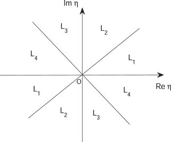
The first column of equation (2.20) enjoys exp $\left[\tfrac{2{\rm{i}}}{\alpha -\beta }{\eta }^{2}(x-\xi )+\tfrac{4{\rm{i}}}{{\left(\alpha -\beta \right)}^{2}}{\eta }^{4}(t-\tau )\right]$, and the following inequalities
$\begin{eqnarray}{\gamma }_{1}\,:x-\xi \geqslant 0,t-\tau \geqslant 0,\end{eqnarray}$
$\begin{eqnarray}{\gamma }_{2}\,:x-\xi \geqslant 0,t-\tau \leqslant 0,\end{eqnarray}$
$\begin{eqnarray}{\gamma }_{3}:x-\xi \leqslant 0,\end{eqnarray}$
are ture on curves ${\{{\gamma }_{j}\}}_{1}^{3}$, then, the bounded analysis area of eigenfunctions ${\{{G}_{j}(x,t,\eta )\}}_{1}^{3}$ is as follows
$\begin{eqnarray}{[{G}_{1}]}_{1}(x,t,\eta )\,:\left\{\mathrm{Im}\displaystyle \frac{{\eta }^{2}}{\alpha -\beta }\geqslant 0\right\}\cap \left\{\mathrm{Im}\displaystyle \frac{{\eta }^{4}}{{\left(\alpha -\beta \right)}^{2}}\geqslant 0\right\},\end{eqnarray}$
$\begin{eqnarray}{[{G}_{2}]}_{1}(x,t,\eta )\,:\left\{\mathrm{Im}\displaystyle \frac{{\eta }^{2}}{\alpha -\beta }\geqslant 0\right\}\cap \left\{\mathrm{Im}\displaystyle \frac{{\eta }^{4}}{{\left(\alpha -\beta \right)}^{2}}\leqslant 0\right\},\end{eqnarray}$
$\begin{eqnarray}{[{G}_{3}]}_{1}(x,t,\eta )\,:\left\{\mathrm{Im}\displaystyle \frac{{\eta }^{2}}{\alpha -\beta }\leqslant 0\right\}.\end{eqnarray}$
On the other hand, the second column of equation (2.20) contains opposite index terms exp $\left[-\tfrac{2{\rm{i}}}{\alpha -\beta }{\eta }^{2}(x-\xi )-\tfrac{4{\rm{i}}}{{\left(\alpha -\beta \right)}^{2}}{\eta }^{4}(t-\tau )\right]$.
$\begin{eqnarray}{[{G}_{1}]}_{1}(x,t,\eta )\,:\left\{\mathrm{Im}\displaystyle \frac{{\eta }^{2}}{\alpha -\beta }\leqslant 0\}\cap \{\mathrm{Im}\displaystyle \frac{{\eta }^{4}}{{\left(\alpha -\beta \right)}^{2}}\leqslant 0\right\},\end{eqnarray}$
$\begin{eqnarray}{[{G}_{2}]}_{1}(x,t,\eta )\,:\left\{\mathrm{Im}\displaystyle \frac{{\eta }^{2}}{\alpha -\beta }\leqslant 0\}\cap \{\mathrm{Im}\displaystyle \frac{{\eta }^{4}}{{\left(\alpha -\beta \right)}^{2}}\geqslant 0\right\},\end{eqnarray}$
$\begin{eqnarray}{[{G}_{3}]}_{1}(x,t,\eta )\,:\left\{\mathrm{Im}\displaystyle \frac{{\eta }^{2}}{\alpha -\beta }\geqslant 0\right\}.\end{eqnarray}$
Consequently, if we remember that ${\left[{G}_{j}\right]}_{k}(x,t,\eta ),k\,=1,2$ represent k-column of Gj(x, t, η), one can get
$\begin{eqnarray}\begin{array}{l}{\rm{for}}\,\alpha \gt \beta ,\\ \left\{\begin{array}{l}{G}_{1}(x,t,\eta )=({\left[{G}_{1}\right]}_{1}^{{L}_{1}}(x,t,\eta ),{\left[{G}_{1}\right]}_{2}^{{L}_{3}}(x,t,\eta )),\\ {G}_{2}(x,t,\eta )=({\left[{G}_{2}\right]}_{1}^{{L}_{2}}(x,t,\eta ),{\left[{G}_{2}\right]}_{2}^{{L}_{4}}(x,t,\eta )),\\ {G}_{3}(x,t,\eta )=({\left[{G}_{3}\right]}_{1}^{{L}_{3}\cup {L}_{4}}(x,t,\eta ),\\ {\left[{G}_{3}\right]}_{2}^{{L}_{1}\cup {L}_{2}}(x,t,\eta )),\end{array}\right.\end{array}\end{eqnarray}$
and
$\begin{eqnarray}\begin{array}{l}{\rm{for}}\,\alpha \lt \beta ,\\ \left\{\begin{array}{l}{G}_{1}(x,t,\eta )=({\left[{G}_{1}\right]}_{1}^{{L}_{4}}(x,t,\eta ),{\left[{G}_{1}\right]}_{2}^{{L}_{2}}(x,t,\eta )),\\ {G}_{2}(x,t,\eta )=({\left[{G}_{2}\right]}_{1}^{{L}_{3}}(x,t,\eta ),{\left[{G}_{2}\right]}_{2}^{{L}_{1}}(x,t,\eta )),\\ {G}_{3}(x,t,\eta )=({\left[{G}_{3}\right]}_{1}^{{L}_{1}\cup {L}_{2}}(x,t,\eta ),\\ {\left[{G}_{3}\right]}_{2}^{{L}_{3}\cup {L}_{4}}(x,t,\eta )),\end{array}\right.\end{array}\end{eqnarray}$
where ${G}_{j}^{{L}_{i}}$ represents that the bounded analytic region of ${\{{G}_{j}\}}_{1}^{3}$ is Li, i = 1, 2, 3, 4, and Li are shown in figure 2.
Figure 2. The areas Lii = 1,…,4 division on the complex η-plane.
To construct the RH problem of GDNLS equation (1.3), we must define another two important special functions $\Psi$(η) and φ(η) by
$\begin{eqnarray}{G}_{3}(x,t,\eta )={G}_{1}(x,t,\eta ){{\rm{e}}}^{-[\tfrac{{\rm{i}}}{\alpha -\beta }{\eta }^{2}x+\displaystyle \frac{2{\rm{i}}}{{\left(\alpha -\beta \right)}^{2}}{\eta }^{4}t]{\hat{\sigma }}_{3}}\psi (\eta ),\end{eqnarray}$
$\begin{eqnarray}{G}_{2}(x,t,\eta )={G}_{1}(x,t,\eta ){{\rm{e}}}^{-[\tfrac{{\rm{i}}}{\alpha -\beta }{\eta }^{2}x+\displaystyle \frac{2{\rm{i}}}{{\left(\alpha -\beta \right)}^{2}}{\eta }^{4}t]){\hat{\sigma }}_{3}}\phi (\eta ),\end{eqnarray}$
upon evaluation at (x, t) = (0, 0) and (x, t) = (0, T), respectively, from equations (2.27a) and (2.27b) we can get
$\begin{eqnarray}{\phi }^{-1}(\eta )={{\rm{e}}}^{-\tfrac{2{\rm{i}}}{{\left(\alpha -\beta \right)}^{2}}{\eta }^{4}T{\hat{\sigma }}_{3}}{G}_{1}(0,T,\eta ),\psi (\eta )={G}_{3}(0,0,\eta ).\end{eqnarray}$
It follows from (2.27a), (2.27b) and equation (2.28) that
$\begin{eqnarray}{G}_{2}(x,t,\eta )={G}_{3}(x,t,\eta ){{\rm{e}}}^{-[\tfrac{{\rm{i}}}{\alpha -\beta }{\eta }^{2}x+\displaystyle \frac{2{\rm{i}}}{{\left(\alpha -\beta \right)}^{2}}{\eta }^{4}t]{\hat{\sigma }}_{3}}{\left(\psi (\eta )\right)}^{-1}\phi (\eta ).\end{eqnarray}$
Particularly, one also obtains G1(x, t, η), G2(x, t, η) at x = 0
$\begin{eqnarray}\begin{array}{rcl}{G}_{1}(0,t,\eta ) & = & ({\left[{G}_{1}\right]}_{1}^{{L}_{1}\cup {L}_{4}}(0,t,\eta ),{\left[{G}_{1}\right]}_{2}^{{L}_{2}\cup {L}_{3}}(0,t,\eta ))\\ & = & {\boldsymbol{I}}+{\displaystyle \int }_{0}^{t}{{\rm{e}}}^{-\tfrac{2{\rm{i}}}{{\left(\alpha -\beta \right)}^{2}}{\eta }^{4}(t-\tau ){\hat{\sigma }}_{3}}({N}_{1}{G}_{1})(0,\tau ,\eta ){\rm{d}}\tau ,\end{array}\end{eqnarray}$
$\begin{eqnarray}\begin{array}{rcl}{G}_{2}(0,t,\eta ) & = & ({\left[{G}_{2}\right]}_{1}^{{L}_{2}\cup {L}_{3}}(0,t,\eta ),{\left[{G}_{2}\right]}_{2}^{{L}_{1}\cup {L}_{4}}(0,t,\eta ))\\ & = & {\boldsymbol{I}}-{\displaystyle \int }_{t}^{T}{{\rm{e}}}^{-\tfrac{2{\rm{i}}}{{\left(\alpha -\beta \right)}^{2}}{\eta }^{4}(t-\tau ){\hat{\sigma }}_{3}}({N}_{1}{G}_{2})(0,\tau ,\eta ){\rm{d}}\tau ,\end{array}\end{eqnarray}$
and G1(xtη), G3(xtη) at t = 0
$\begin{eqnarray}\begin{array}{l}{G}_{1}(x,0,\eta )\\ =\,\left\{\begin{array}{l}({\left[{G}_{1}\right]}_{1}^{{L}_{1}\cup {L}_{2}}(x,0,\eta ),{\left[{G}_{1}\right]}_{2}^{{L}_{3}\cup {L}_{4}}(x,0,\eta ))\,{\rm{for}}\,\alpha \gt \beta ,\\ ({\left[{G}_{1}\right]}_{1}^{{L}_{3}\cup {L}_{4}}(x,0,\eta ),{\left[{G}_{1}\right]}_{2}^{{L}_{1}\cup {L}_{2}}(x,0,\eta ))\,{\rm{for}}\,\alpha \lt \beta ,\end{array}\right.\\ =\,{\boldsymbol{I}}+{\int }_{0}^{x}{{\rm{e}}}^{-\tfrac{{\rm{i}}}{\alpha -\beta }{\eta }^{2}(x-\xi ){\hat{\sigma }}_{3}}({M}_{1}{G}_{1})(\xi ,0,\eta ){\rm{d}}\xi ,\end{array}\end{eqnarray}$
$\begin{eqnarray}\begin{array}{l}{G}_{3}(x,0,\eta )\\ =\,\left\{\begin{array}{l}({\left[{G}_{3}\right]}_{1}^{{L}_{3}\cup {L}_{4}}(z,0,\eta ),{\left[{G}_{3}\right]}_{2}^{{L}_{1}\cup {L}_{2}}(x,0,\eta ))\,{\rm{for}}\,\alpha \gt \beta ,\\ ({\left[{G}_{3}\right]}_{1}^{{L}_{1}\cup {L}_{2}}(z,0,\eta ),{\left[{G}_{3}\right]}_{2}^{{L}_{3}\cup {L}_{4}}(x,0,\eta ))\,{\rm{for}}\,\alpha \lt \beta ,\end{array}\right.\\ =\,{\boldsymbol{I}}-{\int }_{x}^{\infty }{{\rm{e}}}^{-\tfrac{{\rm{i}}}{\alpha -\beta }{\eta }^{2}(x-\xi ){\hat{\sigma }}_{3}}({M}_{1}{G}_{3})(\xi ,0,\eta ){\rm{d}}\xi .\end{array}\end{eqnarray}$
Assume that u0(x) = q(x, t = 0), v0(t) = q(x = 0, t), v1(t) = qx(x = 0, t) are initial condition and boundary conditions of q(x, t) and qx(x, t), then, one get
$\begin{eqnarray}{M}_{1}(x,0,\eta )=\left(\begin{array}{cc}-\displaystyle \frac{{\rm{i}}}{2}(\alpha -\beta )| {u}_{0}{| }^{2} & \eta {\bar{u}}_{0}{{\rm{e}}}^{\tfrac{{\rm{i}}}{2}\alpha {\displaystyle \int }_{0}^{x}| {u}_{0}{| }^{2}{\rm{d}}x}\\ \eta {u}_{0}{{\rm{e}}}^{-\tfrac{{\rm{i}}}{2}\alpha {\displaystyle \int }_{0}^{x}| {u}_{0}{| }^{2}{\rm{d}}x} & \displaystyle \frac{{\rm{i}}}{2}(\alpha -\beta )| {u}_{0}{| }^{2}\end{array}\right),\end{eqnarray}$
$\begin{eqnarray}{N}_{1}(0,t,\eta )=\left(\begin{array}{cc}{N}_{11}^{(1)}(0,t,\eta ) & {N}_{12}^{(1)}(0,t,\eta )\\ {N}_{21}^{(1)}(0,t,\eta ) & -{N}_{11}^{(1)}(0,t,\eta )\end{array}\right),\end{eqnarray}$
with
$\begin{eqnarray*}\begin{array}{rcl}{N}_{11}^{(1)}(0,t,\eta ) & = & -{\rm{i}}{\eta }^{2}| {v}_{0}{| }^{2}-\displaystyle \frac{{\rm{i}}}{8}(2\alpha \beta +{\beta }^{2})| {v}_{0}{| }^{4}\\ & & -\displaystyle \frac{\alpha -\beta }{2}({\bar{v}}_{0}{v}_{1}-{\bar{v}}_{1}{v}_{0}),\\ {N}_{12}^{(1)}(0,t,\eta ) & = & \left(\displaystyle \frac{2}{\alpha -\beta }{\eta }^{3}{\bar{v}}_{0}+\displaystyle \frac{\alpha }{2}| {v}_{0}{| }^{2}{\bar{v}}_{0}-{\rm{i}}{\bar{v}}_{1}\right)\\ & & \times {{\rm{e}}}^{{\rm{i}}{\displaystyle \int }_{0}^{t}\left(\displaystyle \frac{1}{4}({\alpha }^{2}+\alpha \beta -{\beta }^{2})| {v}_{0}{| }^{4}-\displaystyle \frac{{\rm{i}}\alpha }{4}({\bar{v}}_{0}{v}_{1}-{v}_{0}{\bar{v}}_{1})\right){\rm{d}}t},\\ {N}_{21}^{(1)}(0,t,\eta ) & = & \left(\displaystyle \frac{2}{\alpha -\beta }{\eta }^{3}{v}_{0}+\displaystyle \frac{\alpha }{2}| {v}_{0}{| }^{2}{v}_{0}-{\rm{i}}{v}_{1}\right)\\ & & \times {{\rm{e}}}^{-{\rm{i}}{\displaystyle \int }_{0}^{t}\left(\displaystyle \frac{1}{4}({\alpha }^{2}+\alpha \beta -{\beta }^{2})| {v}_{0}{| }^{4}-\displaystyle \frac{{\rm{i}}\alpha }{4}({\bar{v}}_{0}{v}_{1}-{v}_{0}{\bar{v}}_{1})\right){\rm{d}}t}.\end{array}\end{eqnarray*}$

2.3. The other properties of the eigenfunctions

The functions

$\begin{eqnarray*}{G}_{j}(x,t,\eta )=({\left[{G}_{j}\right]}_{1}(x,t,\eta ),{\left[{G}_{j}\right]}_{2}(x,t,\eta )),j=1,2,3,\end{eqnarray*}$
enjoy properties as follows

det Gj(x, t, η) = 1, j = 1,2,3,

${\left[{G}_{1}\right]}_{1}\,{is}\,{analytic}\,{for}$ $\left\{\begin{array}{l}\eta \in {L}_{1},\,{and}\,{continues}\,{to}\,{\bar{L}}_{1},\,\alpha \gt \beta ,\\ \eta \in {L}_{4},\,{and}\,{continues}\,{to}\,{\bar{L}}_{4},\,\alpha \lt \beta ,\end{array}\right.$

${\left[{G}_{1}\right]}_{2}\,{is}\,{analytic}\,{for}$ $\left\{\begin{array}{l}\eta \in {L}_{3},\,{and}\,{continues}\,{to}\,{\bar{L}}_{3},\,\alpha \gt \beta ,\\ \eta \in {L}_{2},\,{and}\,{continues}\,{to}\,{\bar{L}}_{2},\,\alpha \lt \beta ,\end{array}\right.$

${\left[{G}_{2}\right]}_{1}\,{is}\,{analytic}\,{for}$ $\left\{\begin{array}{l}\eta \in {L}_{2},\,{and}\,{continues}\,{to}\,{\bar{L}}_{2},\,\alpha \gt \beta ,\\ \eta \in {L}_{3},\,{and}\,{continues}\,{to}\,{\bar{L}}_{3},\,\alpha \lt \beta ,\end{array}\right.$

${\left[{G}_{2}\right]}_{2}\,{is}\,{analytic}\,{for}$ $\left\{\begin{array}{l}\eta \in {L}_{4},\,{and}\,{continues}\,{to}\,{\bar{L}}_{4},\,\alpha \gt \beta ,\\ \eta \in {L}_{1},\,{and}\,{continues}\,{to}\,{\bar{L}}_{1},\,\alpha \lt \beta ,\end{array}\right.$

${\left[{G}_{3}\right]}_{1}\,{is}\,{analytic}\,{for}$ $\left\{\begin{array}{l}\eta \in {L}_{3}\cup {L}_{4}\,{and}\,{continues}\,{to}\,{\bar{L}}_{3}\cup {\bar{L}}_{4},\alpha \gt \beta ,\\ \eta \in {L}_{1}\cup {L}_{2}\,{and}\,{continues}\,{to}\,{\bar{L}}_{1}\cup {\bar{L}}_{2},\alpha \lt \beta ,\end{array}\right.$

${\left[{G}_{3}\right]}_{2}\,{is}\,{analytic}\,{for}$ $\left\{\begin{array}{l}\eta \in {L}_{1}\cup {L}_{2}\,{and}\,{continues}\,{to}\,{\bar{L}}_{1}\cup {\bar{L}}_{2},\alpha \gt \beta ,\\ \eta \in {L}_{3}\cup {L}_{4}\,{and}\,{continues}\,{to}\,{\bar{L}}_{3}\cup {\bar{L}}_{4},\alpha \lt \beta ,\end{array}\right.$

As η → ∞ , ${\left[{G}_{j}\right]}_{1}(x,t,\eta )\to {\left(\mathrm{1,0}\right)}^{{\rm{T}}}$, ${\left[{G}_{j}\right]}_{2}(x,t,\eta )\to {\left(\mathrm{0,1}\right)}^{{\rm{T}}}.$

Indeed, according to the definition of function Gj(x, t, η) in equation (2.20) and combining with equations (2.25), (2.26), we can easily get this proposition.

To better analyze special functions $\Psi$(η) and φ(η), one can get the following proposition according to the ISM theory.

It follows from equation (2.28) that functions $\Psi$(η), φ(η) can be expressed by

$\begin{eqnarray}\psi (\eta )={\boldsymbol{I}}-{\int }_{0}^{\infty }{{\rm{e}}}^{\tfrac{{\rm{i}}}{\alpha -\beta }{\eta }^{2}(\xi -x){\hat{\sigma }}_{3}}({M}_{1}{G}_{3})(\xi ,0,\eta ){\rm{d}}\xi ,\end{eqnarray}$
$\begin{eqnarray}{\phi }^{-1}(\eta )={\boldsymbol{I}}+{\int }_{0}^{T}{{\rm{e}}}^{\tfrac{2{\rm{i}}}{{\left(\alpha -\beta \right)}^{2}}{\eta }^{4}(\tau -t){\hat{\sigma }}_{3}}({N}_{1}{G}_{1})(0,\tau ,\eta ){\rm{d}}\tau .\end{eqnarray}$

Assume that $\Psi$(η), φ(η) possess the following 2 × 2 matrix from, respectively
$\begin{eqnarray}\psi (\eta )=\left(\begin{array}{cc}\overline{f(\bar{\eta })} & s(\eta )\\ \overline{s(\bar{\eta })} & f(\eta )\end{array}\right),\phi (\eta )=\left(\begin{array}{cc}\overline{F(\bar{\eta })} & S(\eta )\\ \overline{S(\bar{\eta })} & F(\eta )\end{array}\right).\end{eqnarray}$
It follows from equations (2.28) and (2.33a), (2.33b) that the following key properties are ture

$\left(\begin{array}{c}s(\zeta )\\ f(\bar{\zeta })\end{array}\right)={\left[{G}_{3}\right]}_{2}^{{L}_{1}\cup {L}_{2}}(0,0,\eta )$ $=\,\left(\begin{array}{c}{\left({G}_{3}\right)}_{12}^{{L}_{1}\cup {L}_{2}}(0,t,\eta )\\ {\left({G}_{3}\right)}_{22}^{{L}_{1}\cup {L}_{2}}(0,t,\eta )\end{array}\right),$

$\left(\begin{array}{c}-{{\rm{e}}}^{\tfrac{2{\rm{i}}}{{\left(\alpha -\beta \right)}^{2}}{\eta }^{4}T}S(\eta )\\ \overline{F(\bar{\eta })})\end{array}\right)={\left[{G}_{1}\right]}_{2}^{{L}_{2}\cup {L}_{4}}(t,\eta )$ $=\,\left(\begin{array}{c}{\left({G}_{1}\right)}_{12}^{{L}_{2}\cup {L}_{4}}(t,\eta )\\ {\left({G}_{1}\right)}_{22}^{{L}_{2}\cup {L}_{4}}(t,\eta )\end{array}\right),$

f( − η) = f(η),  s( − η) = − s(η), 

F( − η) = F(η),  S( − η) = − S(η), 

$\det \psi (\eta )=f(\eta )\overline{f(\bar{\eta })}-s(\eta )\overline{s(\bar{\eta })}=1,\quad {for}\,\eta \in {\mathbb{R}},$

$\det \phi (\eta )=1,{for}\,\eta \in {\mathbb{C}}\,(\mathrm{Im}\tfrac{2{\eta }^{4}}{{\left(\alpha -\beta \right)}^{2}}=0,{if}\,T=\infty ),$

f(η) = 1 + O(η−1),  s(η) = O(η−1), ${as}\,\eta \to \infty ,\mathrm{Im}\tfrac{{\eta }^{2}}{\alpha -\beta }\gt 0,$

F(η) = 1 + O(η−1),  S(η) = O(η−1), ${as}\,\eta \to \infty ,\mathrm{Im}\tfrac{2{\eta }^{4}}{{\left(\alpha -\beta \right)}^{2}}\gt 0.$

2.4. The basic RH problem

To facilitate subsequent calculations, we remember that the following symbolic assumptions
$\begin{eqnarray}\begin{array}{rcl}\mu (\eta ) & = & \frac{{\eta }^{2}}{\alpha -\beta }x+\frac{2{\eta }^{4}}{{\left(\alpha -\beta \right)}^{2}}t,\\ h(\eta ) & = & f(\eta )\overline{F(\bar{\eta })}-s(\eta )\overline{S(\bar{\eta })},\\ g(\eta ) & = & \overline{f(\bar{\eta })}\overline{S(\bar{\eta })}-\overline{s(\bar{\eta })}\overline{F(\bar{\eta })},\\ \theta (\eta ) & = & \frac{s(\eta )}{\overline{f(\bar{\eta })}},{\rm{\Theta }}(\eta )=-\frac{\overline{S(\bar{\eta })}}{f(\eta )h(\eta )},\end{array}\end{eqnarray}$
then, one obtains
$\begin{eqnarray*}\begin{array}{rcl} & & \overline{S(\bar{\eta })}=f(\eta )g(\eta )+\overline{s(\bar{\eta })}h(\eta ),\\ & & h(\eta )\overline{h(\bar{\eta })}-g(\eta )\overline{g(\bar{\eta })}=1,\\ & & h(-\eta )=h(\eta ),g(-\eta )=-g(\eta ),\\ & & h(\eta )=1+O\left(\displaystyle \frac{1}{\eta }\right),g(\eta )=O\left(\displaystyle \frac{1}{\eta }\right){\rm{as}}\,\eta \to \infty ,\end{array}\end{eqnarray*}$
and the W(x, t, η) is defined by
$\begin{eqnarray}\begin{array}{l}{\rm{for}}\,\alpha \gt \beta ,\\ \left\{\begin{array}{l}{W}_{+}(x,t,\eta )=\left(\tfrac{{\left[{G}_{1}\right]}_{1}^{{L}_{1}}(x,t,\eta )}{f(\eta )},{\left[{G}_{3}\right]}_{2}^{{L}_{1}\cup {L}_{2}}(x,t,\eta )\right),\eta \in {L}_{1},\\ {W}_{-}(x,t,\eta )=\left(\tfrac{{\left[{G}_{2}\right]}_{1}^{{L}_{2}}(x,t,\eta )}{h(\eta )},{\left[{G}_{3}\right]}_{2}^{{L}_{1}\cup {L}_{2}}(x,t,\eta )\right),\eta \in {L}_{2},\\ {W}_{-}(x,t,\eta )=\left({\left[{G}_{3}\right]}_{1}^{{L}_{3}\cup {L}_{4}}(x,t,\eta ),\tfrac{{\left[{G}_{1}\right]}_{2}^{{L}_{3}}(x,t,\eta )}{\overline{f(\bar{\eta })}}\right),\eta \in {L}_{3},\\ {W}_{+}(x,t,\eta )=({\left[{G}_{3}\right]}_{1}^{{L}_{3}\cup {L}_{4}}(x,t,\eta ),\tfrac{{\left[{G}_{2}\right]}_{2}^{{L}_{4}}(x,t,\eta )}{\overline{h(\bar{\eta })}}),\eta \in {L}_{4},\end{array}\right.\end{array}\end{eqnarray}$
$\begin{eqnarray}\begin{array}{l}{\rm{for}}\,\alpha \lt \beta ,\\ \left\{\begin{array}{l}{W}_{+}(x,t,\eta )=\left({\left[{G}_{3}\right]}_{1}^{{L}_{1}\cup {L}_{2}}(x,t,\eta ),\tfrac{{\left[{G}_{2}\right]}_{2}^{{L}_{1}}(x,t,\eta )}{\overline{h(\bar{\eta })}}\right),\eta \in {L}_{1},\\ {W}_{-}(x,t,\eta )=\left({\left[{G}_{3}\right]}_{1}^{{L}_{1}\cup {L}_{2}}(x,t,\eta ),\tfrac{{\left[{G}_{1}\right]}_{2}^{{L}_{2}}(x,t,\eta )}{\overline{f(\bar{\eta })}}\right),\eta \in {L}_{2},\\ {W}_{-}(x,t,\eta )=\left(\tfrac{{\left[{G}_{2}\right]}_{1}^{{L}_{3}}(x,t,\eta )}{h(\eta )},{\left[{G}_{3}\right]}_{2}^{{L}_{3}\cup {L}_{4}}(x,t,\eta )\right),\eta \in {L}_{3},\\ {W}_{+}(x,t,\eta )=\left(\tfrac{{\left[{G}_{1}\right]}_{1}^{{L}_{4}}(x,t,\eta )}{f(\eta )},{\left[{G}_{3}\right]}_{2}^{{L}_{3}\cup {L}_{4}}(x,t,\eta )\right),\eta \in {L}_{4}.\end{array}\right.\end{array}\end{eqnarray}$
These definitions imply that
$\begin{eqnarray}\det W(x,t,\eta )=1,W(x,t,\eta )\to {\boldsymbol{I}},\eta \to \infty .\end{eqnarray}$
In the following, one only gives the case of α > β for jump condition and residue relation, and we can discuss the case of α < β similarly.

For α > β, set $q(x,t)\in {\mathbb{S}}$, and the function W(x, t, η) is given by equation (2.36), then equation (2.36) meets the following jump relation on the curve ${\bar{L}}_{k},k=1,\ldots ,4.$

$\begin{eqnarray}{W}_{-}(x,t,\eta )={W}_{+}(x,t,\eta )H(x,t,\eta ),\eta \in {\bar{L}}_{k},k=1,\ldots ,4,\end{eqnarray}$
where
$\begin{eqnarray}\begin{array}{l}H(x,t,\eta )\\ =\,\left\{\begin{array}{l}{H}_{1}(x,t,\eta ),\qquad \qquad \qquad \arg \tfrac{{\eta }^{2}}{\alpha -\beta }=\tfrac{\pi }{2},\\ {H}_{2}(x,t,\eta )={H}_{3}{H}_{4}^{-1}{H}_{1},\quad \arg \tfrac{{\eta }^{2}}{\alpha -\beta }=\pi ,\\ {H}_{3}(x,t,\eta ),\qquad \qquad \qquad \arg \tfrac{{\eta }^{2}}{\alpha -\beta }=\tfrac{3\pi }{2},\\ {H}_{4}(x,t,\eta ),\qquad \qquad \qquad \arg \tfrac{{\eta }^{2}}{\alpha -\beta }=0,\end{array}\right.\end{array}\end{eqnarray}$
and
$\begin{eqnarray*}\begin{array}{rcl}{H}_{1}(x,t,\eta ) & = & \left(\begin{array}{cc}1 & 0\\ {\rm{\Theta }}(\eta ){{\rm{e}}}^{2{\rm{i}}\mu (\eta )} & 1\end{array}\right),\\ {H}_{3}(x,t,\eta ) & = & \left(\begin{array}{cc}1 & \overline{{\rm{\Theta }}(\bar{\eta })}{{\rm{e}}}^{-2{\rm{i}}\mu (\eta )}\\ 0 & 1\end{array}\right),\\ {H}_{4}(x,t,\eta ) & = & \left(\begin{array}{cc}1 & -\theta (\eta ){{\rm{e}}}^{-2{\rm{i}}\mu (\eta )}\\ \overline{\theta (\bar{\eta })}{{\rm{e}}}^{2{\rm{i}}\mu (\eta )} & 1-| \theta (\eta ){| }^{2}\end{array}\right).\end{array}\end{eqnarray*}$

From equations (2.27a), (2.27b) and (2.34), one finds that

$\begin{eqnarray}\begin{array}{l}\overline{f(\bar{\eta })}{[{G}_{1}]}_{1}^{{L}_{1}}(x,t,\eta )-\overline{s(\bar{\eta })}{{\rm{e}}}^{2{\rm{i}}\mu (\eta )}{[{G}_{1}]}_{2}^{{L}_{3}}(x,t,\eta )\\ \quad =\,{[{G}_{3}]}_{1}^{{L}_{3}\cup {L}_{4}}(x,t,\eta ),\end{array}\end{eqnarray}$
$\begin{eqnarray}\begin{array}{l}s(\eta ){{\rm{e}}}^{-2{\rm{i}}\mu (\eta )}{[{G}_{1}]}_{1}^{{L}_{1}}(x,t,\eta )+f(\eta ){[{G}_{1}]}_{2}^{{L}_{3}}(x,t,\eta )\\ \quad =\,{[{G}_{3}]}_{2}^{{L}_{1}\cup {L}_{2}}(x,t,\eta ),\end{array}\end{eqnarray}$
and
$\begin{eqnarray}\begin{array}{l}\overline{F(\bar{\eta })}{\left[{G}_{1}\right]}_{1}^{{L}_{1}}(x,t,\eta )-\overline{S(\bar{\eta })}{{\rm{e}}}^{2{\rm{i}}\mu (\eta )}{\left[{G}_{1}\right]}_{2}^{{L}_{3}}(x,t,\eta )\\ \quad =\,{\left[{G}_{2}\right]}_{1}^{{L}_{2}}(x,t,\eta ),\end{array}\end{eqnarray}$
$\begin{eqnarray}\begin{array}{l}S(\eta ){{\rm{e}}}^{-2{\rm{i}}\mu (\eta )}{\left[{G}_{1}\right]}_{1}^{{L}_{1}}(x,t,\eta )+F(\eta ){\left[{G}_{1}\right]}_{2}^{{L}_{3}}(x,t,\eta )\\ \quad =\,{\left[{G}_{2}\right]}_{2}^{{L}_{4}}(x,t,\eta ),\end{array}\end{eqnarray}$
then, the equations (2.41a), (2.42b) and (2.35) give rise to
$\begin{eqnarray}\begin{array}{l}h(\eta ){\left[{G}_{3}\right]}_{1}^{{L}_{3}\cup {L}_{4}}(x,t,\eta )-g(\eta ){{\rm{e}}}^{2{\rm{i}}\mu (\eta )}{\left[{G}_{3}\right]}_{2}^{{L}_{1}\cup {L}_{2}}(x,t,\eta )\\ \quad =\,{\left[{G}_{2}\right]}_{1}^{{L}_{2}}(x,t,\eta ),\end{array}\end{eqnarray}$
$\begin{eqnarray}\begin{array}{l}\overline{g(\bar{\eta })}{{\rm{e}}}^{-2{\rm{i}}\mu (\eta )}{\left[{G}_{3}\right]}_{1}^{{L}_{3}\cup {L}_{4}}(x,t,\eta )+\overline{h(\bar{\eta })}{\left[{G}_{3}\right]}_{2}^{{L}_{1}\cup {L}_{2}}(x,t,\eta )\\ \quad =\,{\left[{G}_{2}\right]}_{2}^{{L}_{4}}(x,t,\eta ).\end{array}\end{eqnarray}$
It follows from the equations (2.36) and (2.39) that
$\begin{eqnarray}\begin{array}{l}\left(\displaystyle \frac{{\left[{G}_{1}\right]}_{1}^{{L}_{1}}(x,t,\eta )}{f(\eta )},{\left[{G}_{3}\right]}_{2}^{{L}_{1}\cup {L}_{2}}(x,t,\eta )\right)\\ \quad =\,\left(\displaystyle \frac{{\left[{G}_{2}\right]}_{1}^{{L}_{2}}(x,t,\eta )}{h(\eta )},{\left[{G}_{3}\right]}_{2}^{{L}_{1}\cup {L}_{2}}(x,t,\eta )\right){H}_{1}(x,t,\eta ),\end{array}\end{eqnarray}$
$\begin{eqnarray}\begin{array}{l}\left({\left[{G}_{3}\right]}_{1}^{{L}_{3}\cup {L}_{4}}(x,t,\eta ),\displaystyle \frac{{\left[{G}_{2}\right]}_{2}^{{L}_{4}}(x,t,\eta )}{\overline{h(\bar{\eta })}}\right)\\ \quad =\,\left(\displaystyle \frac{{\left[{G}_{2}\right]}_{1}^{{L}_{2}}(x,t,\eta )}{h(\eta )},{\left[{G}_{3}\right]}_{2}^{{L}_{1}\cup {L}_{2}}(x,t,\eta )\right){H}_{2}(x,t,\eta ),\end{array}\end{eqnarray}$
$\begin{eqnarray}\begin{array}{l}\left({\left[{G}_{3}\right]}_{1}^{{L}_{3}\cup {L}_{4}}(x,t,\eta ),\displaystyle \frac{{\left[{G}_{2}\right]}_{2}^{{L}_{4}}(x,t,\eta )}{\overline{h(\bar{\eta })}}\right)\\ \quad =\,\left({\left[{G}_{3}\right]}_{1}^{{L}_{3}\cup {L}_{4}}(x,t,\eta ),\displaystyle \frac{{\left[{G}_{1}\right]}_{2}^{{L}_{3}}(x,t,\eta )}{\overline{f(\bar{\eta })}}\right){H}_{3}(x,t,\eta ),\end{array}\end{eqnarray}$
$\begin{eqnarray}\begin{array}{l}\left(\displaystyle \frac{{\left[{G}_{1}\right]}_{1}^{{L}_{1}}(x,t,\eta )}{f(\eta )},{\left[{G}_{3}\right]}_{2}^{{L}_{1}\cup {L}_{2}}(x,t,\eta )\right)\\ \quad =\,\left({\left[{G}_{3}\right]}_{1}^{{L}_{3}\cup {L}_{4}}(x,t,\eta ),\displaystyle \frac{{\left[{G}_{1}\right]}_{2}^{{L}_{3}}(x,t,\eta )}{\overline{f(\bar{\eta })}}\right){H}_{4}(x,t,\eta ).\end{array}\end{eqnarray}$
Therefore, the equations (2.44a)–(2.44d) lead to the jump matrices ${\{{H}_{i}(x,t,\eta )\}}_{1}^{4}$ defined by equation (2.40).

One makes assumptions about the simple zeros of functions f(η) and h(η) as follows

f(η) enjoys 2a simple zeros ${\{{\varsigma }_{j}\}}_{j=1}^{2a}$, 2a = 2a1 + 2a2. For α > β, if ${\{{\varsigma }_{j}\}}_{1}^{2{a}_{1}}\in {L}_{1}$, then ${\{{\bar{\varsigma }}_{j}\}}_{1}^{2{a}_{2}}\in {L}_{3}$. For α < β, if ${\{{\varsigma }_{j}\}}_{1}^{2{a}_{1}}\in {L}_{4}$, then ${\{{\bar{\varsigma }}_{j}\}}_{1}^{2{a}_{2}}\in {L}_{2}$.

h(η) enjoys 2b simple zeros ${\{{\zeta }_{j}\}}_{j=1}^{2b}$, 2b = 2b1 + 2b2. For α > β, if ${\{{\zeta }_{j}\}}_{1}^{2{b}_{1}}\in {L}_{4}$, then ${\{{\bar{\zeta }}_{j}\}}_{1}^{2{b}_{2}}\in {L}_{2}$. For α < β, if ${\{{\zeta }_{j}\}}_{1}^{2{b}_{1}}\in {L}_{1}$, then ${\{{\bar{\zeta }}_{j}\}}_{1}^{2{b}_{2}}\in {L}_{3}$.

The intersection of simple zeros of h(η) and f(η) is empty.

(The residue conditions).

Let $\dot{h}(\eta )=\tfrac{{\rm{d}}{h}}{{\rm{d}}\eta }$, one enjoys the following residue conditions:

$\begin{eqnarray}\begin{array}{l}\mathrm{Res}\{{\left[W(x,t,\eta )\right]}_{1},{\varsigma }_{j}\}\\ =\,\displaystyle \frac{1}{s({\varsigma }_{j})\dot{f}({\varsigma }_{j})}{{\rm{e}}}^{2{\rm{i}}\mu ({\varsigma }_{j})}{\left[W(x,t,{\varsigma }_{j})\right]}_{2},j=1,\cdots ,\ 2{a}_{1},\end{array}\end{eqnarray}$
$\begin{eqnarray}\begin{array}{l}\mathrm{Res}\{{\left[W(x,t,\eta )\right]}_{2},{\bar{\varsigma }}_{j}\}\\ =\,-\displaystyle \frac{1}{\overline{s({\varsigma }_{j})}\overline{\dot{f}({\varsigma }_{j})}}{{\rm{e}}}^{-2{\rm{i}}\mu (\bar{{\varsigma }_{j}})}{\left[W(x,t,{\bar{\varsigma }}_{j})\right]}_{1},j=1,\cdots ,\ 2{a}_{2},\end{array}\end{eqnarray}$
$\begin{eqnarray}\begin{array}{l}\mathrm{Res}\{{\left[W(x,t,\eta )\right]}_{1},{\zeta }_{j}\}\\ =\,-\displaystyle \frac{\overline{S({\bar{\zeta }}_{j})}}{f({\zeta }_{j})\dot{h}({\zeta }_{j})}{{\rm{e}}}^{2{\rm{i}}\mu ({\zeta }_{j})}{\left[W(x,t,{\zeta }_{j})\right]}_{1},j=1,\cdots ,\ 2{b}_{1},\end{array}\end{eqnarray}$
$\begin{eqnarray}\begin{array}{l}\mathrm{Res}\{{\left[W(x,t,\eta )\right]}_{2},{\bar{\zeta }}_{j}\}\\ =\,\displaystyle \frac{S({\bar{\zeta }}_{j})}{\overline{f({\zeta }_{j})}\overline{\dot{h}({\zeta }_{j})}}{{\rm{e}}}^{-2{\rm{i}}\mu ({\bar{\zeta }}_{j})}{\left[W(x,t,\bar{{\zeta }_{j}})\right]}_{2},j=1,\cdots ,\ 2{b}_{2}.\end{array}\end{eqnarray}$

One only shows the equation (2.45a). As result of $W(x,t,\eta )=\left(\tfrac{{\left[{G}_{1}\right]}_{1}^{{L}_{1}}}{f(\eta )},{\left[{G}_{3}\right]}_{2}^{{L}_{1}\cup {L}_{2}}\right)$, one finds that the zeros ${\{{\varsigma }_{j}\}}_{1}^{2{a}_{1}}$ of f(η) are the poles of $\tfrac{{\left[{G}_{1}\right]}_{1}^{{L}_{1}}}{f(\eta )}$. Then, one gets

$\begin{eqnarray}\begin{array}{l}\mathrm{Res}\left\{\displaystyle \frac{{G}_{1}^{{L}_{1}}(x,t,\eta )}{f(\eta )},{\varsigma }_{j}\right\}\\ \quad =\,\mathop{\mathrm{lim}}\limits_{\eta \to {\varsigma }_{j}}(\eta -{\varsigma }_{j})\displaystyle \frac{{\left[{G}_{1}\right]}_{1}^{{L}_{1}}(x,t,\eta )}{f(\eta )}=\displaystyle \frac{{\left[{G}_{1}\right]}_{1}^{{L}_{1}}(x,t,{\varsigma }_{j})}{\dot{f}({\varsigma }_{j})},\end{array}\end{eqnarray}$
taking η = ςj into the first and second equations of (2.36), we can get
$\begin{eqnarray}{\left[{G}_{1}\right]}_{1}^{{L}_{1}}(x,t,{\varsigma }_{j})=\displaystyle \frac{1}{s({\varsigma }_{j})}{{\rm{e}}}^{2{\rm{i}}\mu ({\varepsilon }_{j})}{\left[{G}_{3}\right]}_{2}^{{L}_{1}\cup {L}_{2}}(x,t,{\varsigma }_{j}),\end{eqnarray}$
together with equations (2.46) and (2.47), one obtains
$\begin{eqnarray}\begin{array}{l}\mathrm{Res}\left\{\displaystyle \frac{{\left[{G}_{1}\right]}_{1}^{{L}_{1}}(x,t,\eta )}{f(\eta )},{\varsigma }_{j}\right\}\\ \quad =\ \displaystyle \frac{1}{s({\varsigma }_{j})\dot{f}({\varsigma }_{j})}{{\rm{e}}}^{2{\rm{i}}\mu ({\varsigma }_{j})}{\left[{G}_{3}\right]}_{2}^{{L}_{1}\cup {L}_{2}}(x,t,{\varsigma }_{j}),\end{array}\end{eqnarray}$
therefore, the equation (2.48) can lead to the equation (2.45a), and the other three equations (2.45b)–(2.45d) can be similarly proved.

2.5. The inverse problem

The inverse problem includes the reconstruction of potential function q(x, t) from spectral functions ${\{{G}_{j}(x,t,\eta )\}}_{1}^{3}$. It follows from equation (2.10) that ${D}_{1}^{({\rm{od}})}=\tfrac{{\rm{i}}}{2}(\alpha -\beta ){{QD}}_{0}{\sigma }_{3}$. Since asymptotic expansion in equation (2.8) is a solution of equation (2.7), which implies that
$\begin{eqnarray}q(x,t)=-\displaystyle \frac{2{\rm{i}}}{\alpha -\beta }w(x,t){{\rm{e}}}^{-2{\rm{i}}{\int }_{(\mathrm{0,0})}^{(x,t)}{\rm{\Omega }}},\end{eqnarray}$
where G(x, t, η) is related to $\Psi$(x, t, η) as shown in equation (2.15) and given by
$\begin{eqnarray*}\begin{array}{rcl}G(x,t,\eta ) & = & {\boldsymbol{I}}+\displaystyle \frac{{w}^{(1)}(x,t)}{\eta }+\displaystyle \frac{{w}^{(2)}(x,t)}{{\eta }^{2}}\\ & & +O\left(\displaystyle \frac{1}{{\eta }^{3}}\right),\eta \to \infty .\end{array}\end{eqnarray*}$
Meanwhile, G(x, t, η) is the solution of equation (2.16) if ${w}_{21}^{(1)}(x,t)$ replaces of w(x, t). It follows from equation (2.49) and its complex conjugate that
$\begin{eqnarray*}\begin{array}{rcl} & & q\overline{q}=\displaystyle \frac{4}{{\left(\alpha -\beta \right)}^{2}}| w{| }^{2},\\ & & \overline{q}{q}_{x}-q{\overline{q}}_{x}=\displaystyle \frac{4}{{\left(\alpha -\beta \right)}^{2}}(\overline{w}{w}_{x}-w{\overline{w}}_{x})+\displaystyle \frac{8\alpha }{{\left(\alpha -\beta \right)}^{2}}| w{| }^{4}.\end{array}\end{eqnarray*}$
Then, the one-form Ω given by equation (2.13) can be expressed by w(x, t)
$\begin{eqnarray}\begin{array}{rcl}{\rm{\Omega }} & = & \displaystyle \frac{\alpha }{{\left(\alpha -\beta \right)}^{2}}| w{| }^{2}{\rm{d}}x\\ & & -\left[\displaystyle \frac{\alpha }{{\left(\alpha -\beta \right)}^{2}}(\overline{w}{w}_{x}-w{\overline{w}}_{x})-\displaystyle \frac{6\alpha \beta -4{\beta }^{2}}{{\left(\alpha -\beta \right)}^{4}}| w{| }^{4}\right]{\rm{d}}t.\end{array}\end{eqnarray}$
Hence, one can solve the inverse problem according to the following steps successively:
i

(i) One utilizes any one of the functions ${\{{G}_{j}(x,t,\eta )\}}_{1}^{3}$ to calculate w(xt) by

$\begin{eqnarray*}w(x,t)=\mathop{\mathrm{lim}}\limits_{\lambda \to \infty }{\left[\eta {G}_{j}(x,t,\eta )\right]}_{21}.\end{eqnarray*}$

ii

(ii) One gets Ω(xt) from equation (2.50).

iii

(iii) One computes potential function q(xt) by equation (2.49).

2.6. The global relation

In this subsection, one gives the spectral functions f(η), s(η), F(η), S(η) which are not independent but admit a significant relationship. In fact, at the boundary of the region (ξτ): 0 < ξ < ∞, 0 < τ < t, the integral of the one-form A(x, t, η) defined by the equation (2.17) is vanished. Let G(x, t, η) = G3(x, t, η) in the one-form A(x, t, η), one obtains
$\begin{eqnarray}\begin{array}{l}{\displaystyle \int }_{\infty }^{0}{{\rm{e}}}^{\tfrac{{\rm{i}}}{\alpha -\beta }{\eta }^{2}\xi {\hat{\sigma }}_{3}}({M}_{1}{G}_{3})(\xi ,0,\eta ){\rm{d}}\xi \\ \quad +\,{\displaystyle \int }_{0}^{t}{{\rm{e}}}^{\tfrac{2{\rm{i}}}{{\left(\alpha -\beta \right)}^{2}}{\eta }^{4}\tau {\hat{\sigma }}_{3}}({N}_{1}{G}_{3})(0,\tau ,\eta ){\rm{d}}\tau \\ \quad +\,{{\rm{e}}}^{\tfrac{2{\rm{i}}}{{\left(\alpha -\beta \right)}^{2}}{\eta }^{4}t{\hat{\sigma }}_{3}}{\displaystyle \int }_{0}^{\infty }{{\rm{e}}}^{\tfrac{{\rm{i}}}{\alpha -\beta }{\eta }^{2}\xi {\hat{\sigma }}_{3}}({M}_{1}{G}_{3})(\xi ,t,\eta ){\rm{d}}\xi \\ \ =\,\mathop{\mathrm{lim}}\limits_{x\to \infty }{{\rm{e}}}^{\tfrac{{\rm{i}}}{\alpha -\beta }{\eta }^{2}x{\hat{\sigma }}_{3}}{\displaystyle \int }_{0}^{t}{{\rm{e}}}^{\tfrac{2{\rm{i}}}{{\left(\alpha -\beta \right)}^{2}}{\eta }^{4}\tau {\hat{\sigma }}_{3}}({N}_{1}{G}_{3})(x,\tau ,\eta ){\rm{d}}\tau .\end{array}\end{eqnarray}$
On the one hand, since $\Psi$(η) = G3(0, 0, η), together with equation (2.31b), one can find that the first term of the equation (2.51) is
$\begin{eqnarray*}\psi (\eta )-{\boldsymbol{I}}.\end{eqnarray*}$
Set x = 0 in the equation (2.27a), we obtain
$\begin{eqnarray}{G}_{3}(0,\tau ,\eta )={G}_{1}(0,\tau ,\eta ){{\rm{e}}}^{-\tfrac{2{\rm{i}}}{{\left(\alpha -\beta \right)}^{2}}{\eta }^{4}\tau {\hat{\sigma }}_{3}}\psi (\eta ),\end{eqnarray}$
then
$\begin{eqnarray}\begin{array}{l}{{\rm{e}}}^{\tfrac{2{\rm{i}}}{{\left(\alpha -\beta \right)}^{2}}{\eta }^{4}\tau {\hat{\sigma }}_{3}}({N}_{1}{G}_{3})(0,\tau ,\eta )\\ \quad =\,\left[{{\rm{e}}}^{\tfrac{2{\rm{i}}}{{\left(\alpha -\beta \right)}^{2}}{\eta }^{4}\tau {\hat{\sigma }}_{3}}({M}_{1}{G}_{1})(0,\tau ,\eta )\right]\psi (\eta ).\end{array}\end{eqnarray}$
On the other hand, it follows from equations (2.53) and (2.30a) that the second term of the equation (2.51) is
$\begin{eqnarray*}\begin{array}{l}{\displaystyle \int }_{0}^{t}{{\rm{e}}}^{\tfrac{2{\rm{i}}}{{\left(\alpha -\beta \right)}^{2}}{\eta }^{4}\tau {\hat{\sigma }}_{3}}({N}_{1}{G}_{3})(0,\tau ,\eta ){\rm{d}}\tau \\ \quad =\,\left[{{\rm{e}}}^{\tfrac{2{\rm{i}}}{{\left(\alpha -\beta \right)}^{2}}{\eta }^{4}t{\hat{\sigma }}_{3}}{N}_{1}{G}_{1}(0,t,\eta )-I\right]\psi (\eta ).\end{array}\end{eqnarray*}$
Let $q(x,t)\in {\mathbb{S}}$ for x → ∞ , then, equation (2.51) turns into
$\begin{eqnarray}\begin{array}{l}{\phi }^{-1}(t,\eta )\psi (\eta )+{{\rm{e}}}^{\tfrac{2{\rm{i}}}{{\left(\alpha -\beta \right)}^{2}}{\eta }^{4}t{\hat{\sigma }}_{3}}\\ \quad \times \,{\displaystyle \int }_{0}^{\infty }{{\rm{e}}}^{\tfrac{{\rm{i}}}{\alpha -\beta }{\eta }^{2}\xi {\hat{\sigma }}_{3}}({M}_{1}{G}_{3})(\xi ,t,\eta ){\rm{d}}\xi ={\boldsymbol{I}},\end{array}\end{eqnarray}$
where the first column of equation (2.54) is valid for η2 in the lower half-plane and the second column of equation (2.54) is valid for η2 in the upper half-plane, and the expression of φ(t, η) is
$\begin{eqnarray*}{\phi }^{-1}(t,\eta )={{\rm{e}}}^{\tfrac{2{\rm{i}}}{{\left(\alpha -\beta \right)}^{2}}{\eta }^{4}t{\hat{\sigma }}_{3}}{G}_{1}(0,t,\eta ).\end{eqnarray*}$
Denoting φ(η) = φ(Tη) and letting t = T, one finds that the equation (2.54) turns into
$\begin{eqnarray}\begin{array}{l}{\phi }^{-1}(\eta )\psi (\eta )+{{\rm{e}}}^{\tfrac{2{\rm{i}}}{{\left(\alpha -\beta \right)}^{2}}{\eta }^{4}T{\hat{\sigma }}_{3}}\\ \quad \times \,{\displaystyle \int }_{0}^{\infty }{{\rm{e}}}^{\tfrac{{\rm{i}}}{\alpha -\beta }{\eta }^{2}\xi {\hat{\sigma }}_{3}}({M}_{1}{G}_{3})(\xi ,T,\eta ){\rm{d}}\xi ={\boldsymbol{I}}.\end{array}\end{eqnarray}$
Hence, the (21)-component of equation (2.55) is
$\begin{eqnarray}f(\eta )S(\eta )-F(\eta )s(\eta )={{\rm{e}}}^{\tfrac{4{\rm{i}}}{{\left(\alpha -\beta \right)}^{2}}{\eta }^{4}T}E(\eta ),\mathrm{Im}{\eta }^{2}\geqslant 0,\end{eqnarray}$
where E(η) is expressed by
$\begin{eqnarray}E(\eta )={\int }_{0}^{\infty }{{\rm{e}}}^{\tfrac{{\rm{i}}}{\alpha -\beta }{\eta }^{2}\xi }{\left({M}_{1}{G}_{3}\right)}_{21}(\xi ,T,\eta ){\rm{d}}\xi .\end{eqnarray}$
Indeed, equation (2.56) is the so-called global relation.

3. The functions f(η), s(η), F(η) and S(η)

(f(η) and s(η)) Let ${u}_{0}(x)=u(x,0)\in {\mathbb{S}}$, one defines the mapping

$\begin{eqnarray*}{{\mathbb{Y}}}_{1}\,:\{{u}_{0}(x)\}\to \{f(\eta ),s(\eta )\},\end{eqnarray*}$
in terms of
$\begin{eqnarray*}{\left(s(\eta ),f(\eta )\right)}^{{\rm{T}}}=\left\{\begin{array}{l}{[{G}_{3}]}_{2}^{{L}_{1}\cup {L}_{2}}(x,0,\eta ),\,{\rm{for}}\,\alpha \gt \beta ,\\ {[{G}_{3}]}_{2}^{{L}_{3}\cup {L}_{4}}(x,0,\eta ),\,{\rm{for}}\,\alpha \lt \beta ,\end{array}\right.\end{eqnarray*}$
where G3(x, 0, η) is given by
$\begin{eqnarray*}{G}_{3}(x,0,\eta )={\boldsymbol{I}}-{\int }_{x}^{\infty }{{\rm{e}}}^{\tfrac{{\rm{i}}}{\alpha -\beta }{\eta }^{2}(\xi -x){\hat{\sigma }}_{3}}({M}_{1}{G}_{3})(\xi ,0,\eta ){\rm{d}}\xi ,\end{eqnarray*}$
with M1(x, 0, η) expressed by equation (2.32a).

The f(η) and s(η) possess the properties as following

i

(i) f(η), s(η) are analytic and bounded for $\mathrm{Im}\tfrac{1}{\alpha -\beta }{\eta }^{2}\gt 0$ and continuous for $\mathrm{Im}\tfrac{1}{\alpha -\beta }{\eta }^{2}\geqslant 0$.

ii

(ii) $f(\eta )=1\,+\,O\left(\tfrac{1}{\eta }\right),s(\eta )=O\left(\tfrac{1}{\eta }\right)$ as η → ∞, $\mathrm{Im}\tfrac{1}{\alpha -\beta }{\eta }^{2}\geqslant 0$.

iii

(iii) $f(\eta )\overline{f(\bar{\eta })}-s(\eta )\overline{s(\bar{\eta })}=1$, ${\eta }^{2}\in {\mathbb{R}}$.

iv

(iv) f(− η) = f(η), s(− η) = − s(η), $\mathrm{Im}\tfrac{1}{\alpha -\beta }{\eta }^{2}\geqslant 0$.

v

(v) The inverse mapping of ${{\mathbb{Y}}}_{1}$ is ${{\mathbb{Y}}}_{1}^{-1}={{\mathbb{Z}}}_{1}\,:\{f(\eta ),s(\eta )\}\,\to \{{u}_{0}(x)\}$,

which is defined by

$\begin{eqnarray*}\begin{array}{rcl}{u}_{0}(x) & = & -\displaystyle \frac{2{\rm{i}}}{\alpha -\beta }w(x){{\rm{e}}}^{-2{\rm{i}}\alpha {\displaystyle \int }_{0}^{x}| w(\xi ){| }^{2}{\rm{d}}\xi },\\ w(x) & = & \mathop{\mathrm{lim}}\limits_{\eta \to \infty }{\left[\eta {W}^{(x)}(x,\eta )\right]}_{21},\end{array}\end{eqnarray*}$
where W(x)(x, η) admits RH problem as follows.

${W}^{(x)}(x,\eta )=\left\{\begin{array}{l}{W}_{-}^{(x)}(x,\eta ),\mathrm{Im}\tfrac{1}{\alpha -\beta }{\eta }^{2}\leqslant 0,\\ {W}_{+}^{(x)}(x,\eta ),\mathrm{Im}\tfrac{1}{\alpha -\beta }{\eta }^{2}\geqslant 0,\end{array}\right.$ is a section analytic function.

${W}_{-}^{(x)}(x,\eta )={W}_{+}^{(x)}(x,\eta ){\left({H}^{(x)}(x,\eta )\right)}^{-1}$, ${\eta }^{2}\in {\mathbb{R}}$, and

$\begin{eqnarray}{H}^{(x)}(x,\eta )=\left(\begin{array}{cc}1 & -\theta (\eta ){{\rm{e}}}^{-\tfrac{2{\rm{i}}}{\alpha -\beta }{\eta }^{2}x}\\ \overline{\theta (\bar{\eta })}{{\rm{e}}}^{\tfrac{2{\rm{i}}}{\alpha -\beta }{\eta }^{2}x} & 1-| \theta (\eta ){| }^{2}\end{array}\right).\end{eqnarray}$

${W}^{(x)}(x,\eta )={\boldsymbol{I}}+O\left(\tfrac{1}{\eta }\right),\eta \to \infty .$

f(η) possesses 2a simple zeros ${\{{\varsigma }_{j}\}}_{1}^{2a}$, 2a = 2a1 + 2a2, such that $\mathrm{Im}\tfrac{1}{\alpha -\beta }{\varsigma }_{j}^{2}\gt 0,j=1,2,\ \cdots ,\ 2{a}_{1}$, and $\mathrm{Im}\tfrac{1}{\alpha -\beta }{\varsigma }_{j}^{2}\,\lt 0,j=1,2,\ \cdots ,\ 2{a}_{2}$.

The first column of ${W}_{+}^{(x)}(x,\eta )$ enjoys simple poles at $\eta ={\{{\bar{\varsigma }}_{j}\}}_{1}^{2{a}_{2}}$. The second column of ${W}_{-}^{(x)}(x,\eta )$ enjoys simple poles at $\eta ={\{{\varsigma }_{j}\}}_{1}^{2{a}_{1}}$. The relevant residue expression is

$\begin{eqnarray}\begin{array}{l}\mathrm{Res}\{{\left[{W}^{(x)}(x,\eta )\right]}_{1},{\varsigma }_{j}\}\\ \quad =\,\displaystyle \frac{{{\rm{e}}}^{\tfrac{2{\rm{i}}}{\alpha -\beta }{\varsigma }_{j}^{2}x}}{\dot{f}({\varsigma }_{j})s({\varsigma }_{j})}{\left[{W}^{(x)}(x,{\varsigma }_{j})\right]}_{2},j=1,2,\ \cdots ,\ 2{a}_{1},\end{array}\end{eqnarray}$
$\begin{eqnarray}\begin{array}{l}\mathrm{Res}\{{\left[{W}^{(x)}(x,\eta )\right]}_{2},{\bar{\varsigma }}_{j}\}\\ \quad =\displaystyle \frac{{{\rm{e}}}^{-\tfrac{2{\rm{i}}}{\alpha -\beta }{\overline{\varsigma }}_{j}^{2}x}}{\overline{\dot{f}({\varsigma }_{j})}\overline{s({\varsigma }_{j})}}{\left[{W}^{(x)}(x,{\bar{\varsigma }}_{j})\right]}_{1},j=1,2,\ \cdots ,\ 2{a}_{2}.\end{array}\end{eqnarray}$

(i)–(iv) follow from the investigation in section 2.3, and the deduction of (v) can be obtained following [4], where the derivation of u0(x) is given in the inverse problem (see section 2.5).

(F(η) and S(η)) Let ${v}_{0}(t),{v}_{1}(t)\in {\mathbb{S}}$, the mapping

$\begin{eqnarray*}{{\mathbb{Y}}}_{2}\,:\{{v}_{0}(t),{v}_{1}(t)\}\to \{F(\eta ),S(\eta )\},\end{eqnarray*}$
in terms of
$\begin{eqnarray*}{\left(S(\eta ),F(\eta )\right)}^{{\rm{T}}}=\left\{\begin{array}{l}{[{G}_{1}]}_{2}^{{L}_{1}}(x,0,\eta ),\,{\rm{for}}\,\alpha \gt \beta ,\\ {[{G}_{1}]}_{2}^{{L}_{4}}(x,0,\eta ),\,{\rm{for}}\,\alpha \lt \beta ,\end{array}\right.\end{eqnarray*}$
where G1(0, tη) is given by
$\begin{eqnarray*}{G}_{1}(0,t,\eta )={\boldsymbol{I}}-{\int }_{t}^{T}{{\rm{e}}}^{\tfrac{2{\rm{i}}}{{\left(\alpha -\beta \right)}^{2}}{\eta }^{4}(\tau -t){\hat{\sigma }}_{3}}({N}_{1}{G}_{1})(0,\tau ,\eta ){\rm{d}}\tau ,\end{eqnarray*}$
and N1(0, tη) is expressed by equation (2.32b).

The F(η) and S(η) possess the properties as follows

i

(i) F(η), S(η) are analytic and bounded for $\mathrm{Im}\tfrac{2}{{\left(\alpha -\beta \right)}^{2}}{\eta }^{4}\,\geqslant 0$, if T = ∞, the F(η), S(η) are defined only for $\mathrm{Im}\tfrac{2}{{\left(\alpha -\beta \right)}^{2}}{\eta }^{4}\geqslant 0$.

ii

(ii) $F(\eta )=1\,+\,O\left(\tfrac{1}{\eta }\right),S(\eta )=O\left(\tfrac{1}{\eta }\right)$ as η → ∞ , $\mathrm{Im}\tfrac{2}{{\left(\alpha -\beta \right)}^{2}}{\eta }^{4}\geqslant 0$.

iii

(iii) $F(\eta )\overline{F(\bar{\eta })}-S(\eta )\overline{S(\bar{\eta })}=1$, $\eta \in {\mathbb{C}}({\eta }^{4}\in {\mathbb{R}},\,{if}\,T=\infty )$.

iv

(iv) F(−η) = F(η), S(−η) = − S(η), $\mathrm{Im}\tfrac{2}{{\left(\alpha -\beta \right)}^{2}}{\eta }^{4}\geqslant 0$.

v

(v) The inverse mapping of ${{\mathbb{Y}}}_{2}$ is ${{\mathbb{Y}}}_{2}^{-1}={{\mathbb{Z}}}_{2}\,:\{F(\eta ),S(\eta )\}\to \{{v}_{0}(t),{v}_{1}(t)\}$,

which is defined by

$\begin{eqnarray}\begin{array}{rcl}{v}_{0}(t) & = & -\displaystyle \frac{2{\rm{i}}}{\alpha -\beta }{w}_{12}^{(1)}(t){{\rm{e}}}^{-2{\rm{i}}{\displaystyle \int }_{0}^{t}{{\rm{\Omega }}}_{2}(\tau ){\rm{d}}\tau },\\ {v}_{1}(t) & = & \left[\displaystyle \frac{4}{{\left(\alpha -\beta \right)}^{2}}{w}_{21}^{(3)}(t)-{v}_{0}(t){\bar{v}}_{0}(t){w}_{21}^{(1)}(t)\right]{{\rm{e}}}^{-2{\rm{i}}{\displaystyle \int }_{0}^{t}{{\rm{\Omega }}}_{2}(\tau ){\rm{d}}\tau }\\ & & -\displaystyle \frac{2{\rm{i}}}{\alpha -\beta }{v}_{0}(t){w}_{11}^{(2)}(t)-\displaystyle \frac{{\rm{i}}\alpha }{2}| {v}_{0}(t){| }^{2}{\bar{v}}_{0},\end{array}\end{eqnarray}$
where
$\begin{eqnarray*}\begin{array}{rcl}{{\rm{\Omega }}}_{2}(\tau ) & = & 2(-{\alpha }^{2}+\alpha \beta -{\beta }^{2})| {w}_{21}^{(1)}{| }^{4}\\ & & +\displaystyle \frac{2\alpha }{{\left(\alpha -\beta \right)}^{3}}({\bar{w}}_{21}^{(1)}{w}_{21}^{(3)}+{w}_{21}^{(1)}{\bar{w}}_{21}^{(3)})\\ & & -\displaystyle \frac{4\alpha }{\alpha -\beta }| {w}_{21}^{(1)}{| }^{4}-\displaystyle \frac{4\alpha }{\alpha -\beta }| {w}_{21}^{(1)}{| }^{2}\mathrm{Re}[{w}_{11}^{(2)}],\end{array}\end{eqnarray*}$
and the functions w(j)(t), j = 1, 2, 3 are determined by
$\begin{eqnarray*}\begin{array}{rcl}{W}^{(t)}(t,\eta ) & = & {\boldsymbol{I}}+\displaystyle \frac{{w}^{(1)}(t)}{\eta }+\displaystyle \frac{{w}^{(2)}(t)}{{\eta }^{2}}+\displaystyle \frac{{w}^{(3)}(t)}{{\eta }^{3}}\\ & & +O\left(\displaystyle \frac{1}{{\eta }^{4}}\right),\eta \to \infty ,\end{array}\end{eqnarray*}$
where W(t)(t, η) admits RH problem as follows

${W}^{(t)}(t,\eta )=\left\{\begin{array}{ll}{W}_{-}^{(t)}(t,\eta ), & \mathrm{Im}\tfrac{2}{{\left(\alpha -\beta \right)}^{2}}{\eta }^{4}\leqslant 0,\\ {W}_{+}^{(t)}(t,\eta ), & \mathrm{Im}\tfrac{2}{{\left(\alpha -\beta \right)}^{2}}{\eta }^{4}\geqslant 0,\end{array}\right.$ is a section analytic function.

${W}_{-}^{(t)}(t,\eta )={W}_{+}^{(t)}(t,\eta ){H}^{(t)}(t,\eta )$, ${\eta }^{4}\in {\mathbb{R}}$, and

$\begin{eqnarray}{H}^{(t)}(t,\eta )=\left(\begin{array}{cc}1 & -\tfrac{S(\eta )}{\overline{F(\overline{\eta })}}{{\rm{e}}}^{-\tfrac{4{\rm{i}}}{{\left(\alpha -\beta \right)}^{2}}{\eta }^{4}t}\\ \tfrac{\overline{S(\overline{\eta })}}{F(\eta )}{{\rm{e}}}^{\tfrac{4{\rm{i}}}{{\left(\alpha -\beta \right)}^{2}}{\eta }^{4}t} & \tfrac{1}{F(\eta )\overline{F(\overline{\eta })}}\end{array}\right).\end{eqnarray}$

${W}^{(t)}(T,\eta )={\boldsymbol{I}}+O\left(\tfrac{1}{\eta }\right),\eta \to \infty .$

F(η) possesses 2k simple zeros ${\{{\varepsilon }_{j}\}}_{1}^{2k}$, 2k = 2k1 + 2k2 such that $\mathrm{Im}\tfrac{2}{{\left(\alpha -\beta \right)}^{2}}{\varepsilon }_{j}^{4}\gt 0,j\,=\,1,2,\cdots ,2{k}_{1}$, and $\mathrm{Im}\tfrac{2}{{\left(\alpha -\beta \right)}^{2}}{\varepsilon }_{j}^{4}\lt 0,j\,=\,1,2,\cdots ,2{k}_{2}$.

The first column of ${W}_{+}^{(t)}(t,\eta )$ enjoys simple poles at $\eta ={\{{\bar{\varepsilon }}_{j}\}}_{1}^{2{k}_{2}}$, the second column of ${W}_{-}^{(t)}(t,\eta )$ enjoys simple poles at $\eta ={\{{\varepsilon }_{j}\}}_{1}^{2{k}_{2}}$. The relevant residue expression is

$\begin{eqnarray}\begin{array}{l}\mathrm{Res}\{{\left[{W}^{(t)}(t,\eta )\right]}_{1},{\varepsilon }_{j}\}\\ =\,\displaystyle \frac{{{\rm{e}}}^{\tfrac{4{\rm{i}}}{{\left(\alpha -\beta \right)}^{2}}{\varepsilon }_{j}^{4}t}}{\dot{F}({\varepsilon }_{j})S({\varepsilon }_{j})}{\left[{W}^{(t)}(t,{\varepsilon }_{j})\right]}_{2},j=1,2,\cdots ,2{k}_{1},\end{array}\end{eqnarray}$
$\begin{eqnarray}\begin{array}{l}\mathrm{Res}\{{\left[{W}^{(t)}(t,\eta )\right]}_{2},{\bar{\varepsilon }}_{j}\}\\ =\,\displaystyle \frac{{{\rm{e}}}^{-\tfrac{4{\rm{i}}}{{\left(\alpha -\beta \right)}^{2}}{\overline{\varepsilon }}_{j}^{4}t}}{\overline{\dot{F}({\bar{\varepsilon }}_{j})}\overline{S({\bar{\varepsilon }}_{j})}}{\left[{W}^{(t)}(t,{\bar{\varepsilon }}_{j})\right]}_{1},j=1,2,\ \cdots ,\ 2{k}_{2}.\end{array}\end{eqnarray}$

(i)–(iv) follow from the investigate in section 2.3, and the deduction of (v) can be obtained following [4], where the derivation of v0(t) and v1(t) are given in appendix.

4. The RH problem

Let ${u}_{0}(x)\in {\mathbb{S}}({{\rm{R}}}^{+})$, the matrix functions $\Psi$(η) and φ(η) in terms of f(η), s(η), F(η), S(η) are given by equation (2.34), respectively. Assume that the possible simple zeros ${\{{\varsigma }_{j}\}}_{j=1}^{2a}$ of function f(η) and ${\{{\zeta }_{j}\}}_{j=1}^{2b}$ of function h(η) are given by assumption 2.4. Therefore, the matrix-value function W(x, t, η) conforms to the following RH problem:

W(xtη) is the slice analytic function for η ∈ Lk and continuous to ${\bar{L}}_{k},(k=1,\ \ldots ,\ 4)$.

W(xtη) jump arises on the curves ${\{{\bar{L}}_{k}\}}_{1}^{4}$ and admits the jump relation given by theorem 2.3, i.e.

$\begin{eqnarray*}{W}_{-}(x,t,\eta )={W}_{+}(x,t,\eta )H(x,t,\eta ),\eta \in {\bar{L}}_{k},k=1,\ \ldots ,\ 4,\end{eqnarray*}$

$W(x,t,\eta )={\boldsymbol{I}}+{\rm{O}}\left(\tfrac{1}{\eta }\right),\eta \to \infty $.

W(xtη) meets the residue conditions given by proposition 2.5.

Hence, the function W(xtη) is uniquely existing. Then, one can use W(xtη) to define q(xt) as
$\begin{eqnarray}\begin{array}{rcl} & & q(x,t)=-\displaystyle \frac{2{\rm{i}}}{\alpha -\beta }w(x,t){{\rm{e}}}^{-2{\rm{i}}{\displaystyle \int }_{(\mathrm{0,0})}^{(x,t)}{\rm{\Omega }}},\\ & & w(x,t)=\mathop{\mathrm{lim}}\limits_{\eta \to \infty }{\left[\eta W(x,t,\eta )\right]}_{21},\\ & & {\rm{\Omega }}=\displaystyle \frac{\alpha }{{\left(\alpha -\beta \right)}^{2}}| w{| }^{2}{\rm{d}}x\\ & & -\left[\displaystyle \frac{\alpha }{{\left(\alpha -\beta \right)}^{2}}(\overline{w}{w}_{x}-w{\overline{w}}_{x})-\displaystyle \frac{6\alpha \beta -4{\beta }^{2}}{{\left(\alpha -\beta \right)}^{4}}| w{| }^{4}\right]{\rm{d}}t,\end{array}\end{eqnarray}$
thus, the function q(x, t) is a solution of the GDNLS equation (1.3). Furthermore, u(x, 0) = u0(x),  u(0, t) = v0(t), ux(0, t) = v1(t). 

Indeed, one can manifest the above RH problem following [4].

5. Conclusions and discussions

In this paper, we use UTM to discuss the IBVPs of the generalized DNLS equation (1.3), one can also discuss the equation (1.3) on a finite interval, and analyze the asymptotic behavior of the solution for the equation (1.3) by the Deift–Zhou method [36]. Since the RH problem is equivalent to Gel’fand–Levitan–Marchenko (GLM) theory, one can obtain the soliton solution of the equation (1.3) by solving the GLM equation following [37], which are our future investigation work.

Acknowledgments

This work is supported by the Natural Science Foundation of China (Nos. 11 601 055, 11 805 114 and 11 975 145), the Natural Science Research Projects of Anhui Province (No. KJ2019A0637), and University Excellent Talent Fund of Anhui Province (No. gxyq2019096).

Appendix. Recovering v0(t) and v1(t)

In this appendix, we will give a proof of equation (3.3), that is, derive v0(t) and v1(t) from W(t). Let G(x, t, η) is a solution of equation (2.16). According to equation (2.11), one gets
$\begin{eqnarray}\begin{array}{rcl}{\rm{i}}{Q}_{x}{\sigma }_{3}{D}_{0} & = & \displaystyle \frac{4{\rm{i}}}{{\left(\alpha -\beta \right)}^{2}}{D}_{4}^{({\rm{od}})}{\sigma }_{3}-{\rm{i}}{Q}^{2}{\sigma }_{3}{D}_{2}^{({\rm{od}})}\\ & & +\displaystyle \frac{2}{\alpha -\beta }{{QD}}_{3}^{(d)}+\displaystyle \frac{\alpha }{2}{Q}^{3}{D}_{0},\end{array}\end{eqnarray}$
where $\Psi$(x, t, η) is the solution of equation (2.7) and enjoys the following form
$\begin{eqnarray*}{\rm{\Psi }}(x,t,\eta )={D}_{0}+\displaystyle \frac{{D}_{1}}{\eta }+\displaystyle \frac{{D}_{2}}{{\eta }^{2}}+\displaystyle \frac{{D}_{3}}{{\eta }^{3}}+O\left(\displaystyle \frac{1}{{\eta }^{4}}\right),\eta \to \infty .\end{eqnarray*}$
Since $\Psi$(x, t, η) is defined by equation (2.15) and related to G(x, t, η) as follows
$\begin{eqnarray*}G(x,t,\eta )=\left(\begin{array}{cc}{G}_{11} & {G}_{12}\\ {G}_{21} & {G}_{22}\end{array}\right),\end{eqnarray*}$
then, one gets
$\begin{eqnarray*}{\rm{\Psi }}(x,t,\eta )=\left(\begin{array}{cc}{D}_{0}^{11}{G}_{11} & {D}_{0}^{22}{{\rm{e}}}^{2{\rm{i}}{\displaystyle \int }_{(\mathrm{0,0})}^{(x,t)}{\rm{\Omega }}}{G}_{12}\\ {D}_{0}^{11}{{\rm{e}}}^{-2{\rm{i}}{\displaystyle \int }_{(\mathrm{0,0})}^{(x,t)}{\rm{\Omega }}}{G}_{21} & {D}_{0}^{22}{G}_{22}\end{array}\right).\end{eqnarray*}$
If seeking
$\begin{eqnarray*}G(x,t,\eta )={\boldsymbol{I}}+\displaystyle \frac{{w}^{(1)}}{\eta }+\displaystyle \frac{{w}^{(2)}}{{\eta }^{2}}+\displaystyle \frac{{w}^{(3)}}{{\eta }^{3}}+O\left(\displaystyle \frac{1}{{\eta }^{4}}\right),\eta \to \infty ,\end{eqnarray*}$
then the (21)-entry of equation (A.1) gives
$\begin{eqnarray}\begin{array}{rcl}{q}_{x} & = & \left[\displaystyle \frac{4}{{\left(\alpha -\beta \right)}^{2}}{w}_{21}^{(3)}-q\bar{q}{w}_{21}^{(1)}\right]{{\rm{e}}}^{-2{\rm{i}}{\displaystyle \int }_{(\mathrm{0,0})}^{(x,t)}{\rm{\Omega }}}\\ & & -\displaystyle \frac{2{\rm{i}}}{\alpha -\beta }{{qw}}_{11}^{(2)}-\displaystyle \frac{{\rm{i}}\alpha }{2}{q}^{2}\bar{q}.\end{array}\end{eqnarray}$
Taking the complex conjugate yields
$\begin{eqnarray}\begin{array}{rcl}{\bar{q}}_{x} & = & \left[\displaystyle \frac{4}{{\left(\alpha -\beta \right)}^{2}}{\bar{w}}_{21}^{(3)}-q\bar{q}{\bar{w}}_{21}^{(1)}\right]{{\rm{e}}}^{2{\rm{i}}{\displaystyle \int }_{(\mathrm{0,0})}^{(x,t)}{\rm{\Omega }}}\\ & & +\displaystyle \frac{2{\rm{i}}}{\alpha -\beta }\bar{q}{\bar{w}}_{11}^{(2)}+\displaystyle \frac{{\rm{i}}\alpha }{2}q{\bar{q}}^{2}.\end{array}\end{eqnarray}$
At the same time, from equation (2.49), one finds
$\begin{eqnarray}\begin{array}{rcl}q(x,t) & = & -\displaystyle \frac{2{\rm{i}}}{\alpha -\beta }{w}_{21}^{(1)}{{\rm{e}}}^{-2{\rm{i}}{\displaystyle \int }_{(\mathrm{0,0})}^{(x,t)}{\rm{\Omega }}},\\ \bar{q}(x,t) & = & \displaystyle \frac{2{\rm{i}}}{\alpha -\beta }{\bar{w}}_{21}^{(1)}{{\rm{e}}}^{2{\rm{i}}{\displaystyle \int }_{(\mathrm{0,0})}^{(x,t)}{\rm{\Omega }}}.\end{array}\end{eqnarray}$
It follows from equations (A.2)–(A.4) that
$\begin{eqnarray}\begin{array}{l}\bar{q}{q}_{x}-q{\bar{q}}_{x}=\displaystyle \frac{8{\rm{i}}}{{\left(\alpha -\beta \right)}^{3}}({\bar{w}}_{21}^{(1)}{w}_{21}^{(3)}+{w}_{21}^{(1)}{\bar{w}}_{21}^{(3)})\\ -\,\displaystyle \frac{4{\rm{i}}}{\alpha -\beta }q\bar{q}{w}_{21}^{(1)}{\bar{w}}_{21}^{(1)}-\displaystyle \frac{4{\rm{i}}}{\alpha -\beta }q\bar{q}\mathrm{Re}[{w}_{11}^{(2)}]-{\rm{i}}\alpha {q}^{2}{\bar{q}}^{2},\end{array}\end{eqnarray}$
which means that the coefficient ${{\rm{\Omega }}}_{2}=\tfrac{1}{8}({\alpha }^{2}+\alpha \beta \,-{\beta }^{2})| q{| }^{4}-\tfrac{{\rm{i}}}{4}\alpha (\bar{q}{q}_{x}-q{\bar{q}}_{x})$ of dt in the differential form Ω defined in equation (2.14) can be expressed as
$\begin{eqnarray}\begin{array}{rcl}{{\rm{\Omega }}}_{2} & = & \displaystyle \frac{1}{8}(-{\alpha }^{2}+\alpha \beta -{\beta }^{2})| q{| }^{4}\\ & & +\displaystyle \frac{2\alpha }{{\left(\alpha -\beta \right)}^{3}}({\bar{w}}_{21}^{(1)}{w}_{21}^{(3)}+{w}_{21}^{(1)}{\bar{w}}_{21}^{(3)})\\ & & -\displaystyle \frac{\alpha }{\alpha -\beta }q\bar{q}{w}_{21}^{(1)}{\bar{w}}_{21}^{(1)}-\displaystyle \frac{\alpha }{\alpha -\beta }q\bar{q}\mathrm{Re}[{w}_{11}^{(2)}].\end{array}\end{eqnarray}$
Owing to $q\bar{q}=4| {w}_{21}^{(1)}{| }^{2},$ we calculate equations (A.2), (A.4)–(A.7) at x = 0 and yield
$\begin{eqnarray}\begin{array}{rcl}{v}_{0}(t) & = & -\displaystyle \frac{2{\rm{i}}}{\alpha -\beta }{w}_{12}^{(1)}(t){{\rm{e}}}^{-2{\rm{i}}{\displaystyle \int }_{0}^{t}{{\rm{\Omega }}}_{2}(\tau ){\rm{d}}\tau },\\ {v}_{1}(t) & = & \left[\displaystyle \frac{4}{{\left(\alpha -\beta \right)}^{2}}{w}_{21}^{(3)}(t)-{v}_{0}(t){\bar{v}}_{0}(t){w}_{21}^{(1)}(t)\right]{{\rm{e}}}^{-2{\rm{i}}{\displaystyle \int }_{0}^{t}{{\rm{\Omega }}}_{2}(\tau ){\rm{d}}\tau }\\ & & -\displaystyle \frac{2{\rm{i}}}{\alpha -\beta }{v}_{0}(t){w}_{11}^{(2)}(t)-\displaystyle \frac{{\rm{i}}\alpha }{2}| {v}_{0}(t){| }^{2}{\bar{v}}_{0},\end{array}\end{eqnarray}$
with
$\begin{eqnarray}\begin{array}{rcl}{{\rm{\Omega }}}_{2}(\tau ) & = & 2(-{\alpha }^{2}+\alpha \beta -{\beta }^{2})| {w}_{21}^{(1)}{| }^{4}\\ & & +\displaystyle \frac{2\alpha }{{\left(\alpha -\beta \right)}^{3}}({\bar{w}}_{21}^{(1)}{w}_{21}^{(3)}+{w}_{21}^{(1)}{\bar{w}}_{21}^{(3)})\\ & & -\displaystyle \frac{4\alpha }{\alpha -\beta }| {w}_{21}^{(1)}{| }^{4}-\displaystyle \frac{4\alpha }{\alpha -\beta }| {w}_{21}^{(1)}{| }^{2}\mathrm{Re}[{w}_{11}^{(2)}],\end{array}\end{eqnarray}$
where the functions w(j)(t), j = 1, 2, 3 are determined by
$\begin{eqnarray}\begin{array}{rcl}{W}^{(t)}(t,\eta ) & = & {\boldsymbol{I}}+\displaystyle \frac{{w}^{(1)}(t)}{\eta }+\displaystyle \frac{{w}^{(2)}(t)}{{\eta }^{2}}+\displaystyle \frac{{w}^{(3)}(t)}{{\eta }^{3}}\\ & & +O\left(\displaystyle \frac{1}{{\eta }^{4}}\right),\eta \to \infty .\end{array}\end{eqnarray}$
1
Gardner C S Green J M Kruskal M D Miüra R M 1967 Phys. Rev. Lett. 19 1095 1097

DOI

2
Fokas A S 1997 Proc. R. Soc. A 453 1411 1443

DOI

3
Fokas A S Its A R Sung L Y 2005 Nonlinearity 18 1771 1822

DOI

4
Lenells J 2008 Physica D 237 3008 3019

DOI

5
Mjolhus E 1976 J. Plasma Phys. 16 321 334

DOI

6
Kaup D J Newell A C 1978 J. Math. Phys. 19 789 801

DOI

7
Feng Z S Wang X H 2001 Phys. Scr. 64 7 14

DOI

8
Wadati M Konno K Ichikawa Y H 1979 J. Phys. Soc. Jpn. 46 1965 1966

DOI

9
Kundu A 1984 J. Math. Phys. 25 3433 3438

DOI

10
Lenells J 2011 Commun. Math. Phys. 304 585 635

DOI

11
Zhang N Xia T C Hu B B 2017 Commun. Theor. Phys. 68 580 594

DOI

12
Xia B Q Fokas A S 2018 Physica D 364 27 61

DOI

13
Ai L P Xu J 2019 Appl. Math. Lett. 87 57 63

DOI

14
Zhang Y S Rao J G Cheng Y He J S 2019 Physica D 399 173 185

DOI

15
Chen S Y Yan Z Y 2019 Appl. Math. Lett. 95 65 71

DOI

16
Huang L 2020 Chin. Ann. Math. Ser. B 41 117 132

DOI

17
Hu B B Zhang L Xia T C Zhang N 2020 Appl. Math. Comput. 381 125262

DOI

18
Xu J Fan E G 2014 Acta Math. Sci. 34 973 994

DOI

19
Lenells J 2012 Physica D 241 857 875

DOI

20
Lenells J 2013 Nonlinear Anal. 76 122 139

DOI

21
Monvel A B Shepelsky D 2013 Nonlinearity 26 2081 2107

DOI

22
Xu J Fan E G 2013 Proc. R. Soc. A 469 20130068

DOI

23
Xu J Fan E G 2014 Phys. Lett. A 378 26 33

DOI

24
Tian S F 2019 J. Differ. Equ. 262 506 558

DOI

25
Yan Z Y 2019 J. Math. Phys. 60 1 70

DOI

26
Hu B B Xia T C Zhang N Wang J B 2018 Int. J. Nonlinear Sci. Numer. 19 83 92

DOI

27
Hu B B Xia T C 2019 Complex Var. Elliptic 64 2019 2039

DOI

28
Wang D S Wang X L 2018 Nonlinear Anal. Real. 41 334 361

DOI

29
Yang B Chen Y 2019 Nonlinear Anal. Real. 45 918 941

DOI

30
Ma W X 2019 Nonlinear Anal. Real. 47 1 17

DOI

31
Clarkson P A Cosgrove C M 1987 J. Phys. A: Math. Gen. 20 2003 2024

DOI

32
Clarkson P A 1992 Nonlinearity 5 453 472

DOI

33
Wyller J Fl T Rasmussen J J 1998 Phys. Scr. 57 427 435

DOI

34
Zhang N Xia T C Fan E G 2018 Acta Math. Appl. Sin. 34 493 515

DOI

35
X Peng M S 2013 Commun. Nonlinear Sci. Numer. Simul. 18 2304 2312

DOI

36
Deift P A Zhou X 1993 Ann. Math. 137 295 368

DOI

37
Zhang Y S Xu S W 2020 Appl. Math. Lett. 99 105995

DOI

Outlines

/