


1. Introduction
An electric field associated with magnetospheric wave phenomena was first suggested by Alfven and Falthammar [1] on the basis of theoretical arguments, and has been an important feature of auroral plasma over the past couple of decades. Numerous observations from magnetospheric plasma reveal that such an electric field predominantly occurs along the Earth’s magnetic field [2–6]. Auroral observations by the Viking satellite have shown that the time duration of electric fields are a few tens of seconds and their values are from a few to 20 mV m−1 [7]. Based on the observations of the electric field associated with electrostatic shocks and double layers from the auroral zone, Temerin and Mozer [8] inferred that the average peak value of parallel electric fields is 25 mV m−1. However, observations from the auroral region also reveal that electric fields are found with amplitudes more than 100 mV m−1, but these electric fields are restricted to relatively small regions [9, 10]. Mozer and Kletzing [11] reported the direct observations of large amplitude electric fields of more than 100 mV m−1 from the upward current auroral region. From the upward current auroral region, the direct observations of parallel electric fields pointed out the localization of these fields almost up to 10 Debye lengths [12]. Furthermore, Schriver and Ashour-Abdulla [13] reported that large- and small-scale electric fields exist in the auroral region. Shi et al [14] studied the nonlinear electrostatic waves in the context of auroral plasma and suggested that bipolar electric field solitary structures could be the result of nonlinear evolution of such electrostatic waves. Therefore, the existence of an electric field parallel to the magnetic field in the auroral region has now been well established.
The presence of an electric field and electrodynamical coupling of the ionosphere and magnetosphere have a significant effect on the regional electrodynamics and transportation of charged particles. One of the commonly observed electromagnetic waves in the magnetosphere is electromagnetic electron cyclotron (EMEC) waves. The electron temperature anisotropy and streaming electrons are supposed to be the cause of excitation of these waves [15]. Whistler waves are the low-frequency branch of the full spectrum of EMEC waves that have been observed extensively in terrestrial foreshock, magnetosheath and magnetosphere [16]. The presence of the electric field may affect the morphological characteristics of whistler waves generated by the wave particle interaction. By employing the bi-Maxwellian distribution, Misra and Singh [17] found out how EMEC waves are amplified by electric fields in weakly ionized Maxwellian plasma, but this work was restricted to a small value of temperature anisotropy. In the auroral region, for large values of temperature anisotropies, Renuka and Viswanathan [18] investigated the EMEC instability in a plasma which consists of a nonthermal cold component and Maxwellian hot component. It is worth noting that we employ kappa-Maxwellian distribution function, whereas in [17, 18] bi-Maxwellian was used. Excitation of whistler waves has also been studied in low-altitude auroral plasma, comprising cold and trapped energetic electrons with ${n}_{e}\lt {n}_{c},$ where ${n}_{e}$ and ${n}_{c}$ are the energetic and cold electron densities [19]. This study showed that the downward propagating whistler waves could be produced by dint of cyclotron maser instability at the low-altitude auroral region of about 600 km. Later, Wu et al [20] studied EMEC instability by taking arbitrary values of ${n}_{e}/{n}_{c}$ for varying altitudes of the auroral region. The energetic electrons (∼1 keV) belonging to the plasma sheet region were transported along the magnetic field lines to the auroral region during the magnetic substorm and got trapped there because of the presence of the parallel electric field at high altitude and magnetic mirror effect at low-altitude regions, respectively [21–23]. The plasma comprising such energetic particles shows significant deviation from Maxwellian distribution and can thus could be well be modeled by non-Maxwellian distribution functions. A general non-Maxwellian distribution which is used to model the high-energy tail of the distribution is the kappa distribution [24, 25]. A more general non-Maxwellian distribution is the generalized $(r,q)$ distribution, which is used as a model not only for high-energy particles but for particles at low energies as well [26–28]. Whistler instability has been studied by employing bi-kappa distribution, and found a strong dependence of maximum growth rate on $\kappa $-index, but it was noted that $\kappa $ does not affect the threshold condition [29]. Whistler instability has also been studied by employing bi-$(r,q)$ distribution, and again found strong dependence of maximum growth rate on $r,q$ indices [30]. Later, whistler instability has also been investigated by Lazar et al [31] using bi-kappa distribution, and found a strong dependence of threshold condition on $\kappa $-index for maximum growth rate. By employing kappa-Maxwellian distribution ($\kappa M$), which is another non-Maxwellian distribution, in which the perpendicular part was represented by Maxwellian and the parallel part by kappa, Hellberg and Mace [32] investigated the electrostatic waves and derived the general dispersion function for such a distribution. Cattaert et al [33] investigated the electromagnetic waves propagating obliquely in magneto-plasma characterized by $\kappa M$-distribution. Furthermore, electromagnetic ion cyclotron (EMIC) waves have been studied in five-component plasma by employing $\kappa M$-distribution for hot protons [34]. EMEC waves have been studied in Maxwellian auroral plasma in the presence of a parallel electric field [35]. By employing Maxwellian and non-Maxwellian electron distributions, different authors have studied the excitation of EMEC waves in the absence of a parallel electric field [36–38]. Recently, Nazeer et al [39] studied EMEC waves by employing $\kappa M$-distribution for auroral trapped electrons.
In this paper, using linear kinetic theory, EMEC instability has been studied to explore the interplay of trapped electron speed and parallel electric field in the context of $\kappa M$- distributed auroral plasma. The growth rate for EMEC instability has been derived using the $\kappa M$-distribution for arbitrary values of trapped electron density and various altitudes. A theoretical model and the derivation of dispersion relation for EMEC waves in $\kappa M$-plasma are presented in section 2 . In section 3 , we present the numerical solution and effect on the growth rate studied by changing the different plasma parameters. Finally, we present our conclusions in section 4 .
2. Model formulism
In this paper, we assume uniform, collisionless and anisotropic plasma comprising cold ionospheric background electrons and trapped energetic (hot) electrons in the presence of a parallel electric field which is a salient feature of auroral plasma. These energetic trapped electrons exhibit a bump along the perpendicular axis in velocity space [20]. Moreover, we consider ion population as immobile providing neutralizing background; therefore, ion dynamics is completely neglected. The $\kappa M$-distribution function is considered as a model distribution for trapped energetic electrons in which $\kappa $-distribution is used to model the parallel accelerated motion and perpendicular motion is modeled by Maxwellian distribution. Thus the distribution function for trapped electrons is written as [39]3 ) is modified due to the presence of the parallel electric field, and has the form
$\begin{eqnarray}\begin{array}{l}{f}_{{\rm{\kappa }}M}\left({v}_{\parallel },{v}_{\perp }\right)=\displaystyle \frac{{n}_{e}/n}{A\,{\pi }^{3/2}{\theta }_{\perp }^{2}{\theta }_{\parallel c}}\displaystyle \frac{{\rm{\Gamma }}\left(\kappa +1\right)}{{\kappa }^{3/2}{\rm{\Gamma }}\left(\kappa -\tfrac{1}{2}\right)}\\ \,\times \,{\left(1+\displaystyle \frac{{{v}_{\parallel }}^{2}}{\kappa {\theta }_{\parallel c}^{2}}\right)}^{-\kappa }\exp \left\{-\,\displaystyle \frac{{\left({v}_{\perp }-{v}_{0}\right)}^{2}}{{\theta }_{\perp }^{2}}\right\},\end{array}\end{eqnarray}$
where $\begin{eqnarray}A=\exp \left[-\displaystyle \frac{{{v}_{0}}^{2}}{{{\theta }_{\perp }}^{2}}\right]+\sqrt{\pi }\displaystyle \frac{{v}_{0}}{{\theta }_{\perp }}\,\mathrm{erfc}\left(-\displaystyle \frac{{v}_{0}}{{\theta }_{\perp }}\right).\end{eqnarray}$
Here ${n}_{e}$ is the energetic electron and $n$ is the total electron density, ${v}_{0}$ is the mean energetic trapped electrons drift speed in the perpendicular direction defined as ${v}_{0}=\displaystyle {\int }_{0}^{\infty }{v}_{0}f\left({v}_{\perp }\right){v}_{\perp }{\rm{d}}{v}_{\perp },$ where $f\left({v}_{\perp }\right)=F(s)$ with $s=({v}_{\perp }-{v}_{0})$/${\theta }_{\perp },$ ${\rm{Erfc}}()$ is the complementary error function, and $\begin{eqnarray}{T}_{\parallel }=\displaystyle \frac{m\,{\theta }_{\parallel c}^{2}}{2}\left(\displaystyle \frac{\kappa }{\kappa -3/2}\right),\end{eqnarray}$
$\begin{eqnarray}{T}_{\perp }=\displaystyle \frac{m\,{\theta }_{\perp }^{2}}{2\,}\left(1+\,\displaystyle \frac{{v}_{0}^{2}}{{\theta }_{\perp }^{2}}\,+\,\displaystyle \frac{\sqrt{\pi }\,{v}_{0}}{2\,A\,{\theta }_{\perp }}\,\mathrm{erfc}\left(-\,\displaystyle \frac{{v}_{0}}{{\theta }_{\perp }}\right)\right)\end{eqnarray}$
are the modified parallel and perpendicular electron temperatures, respectively. Here we note that the parallel thermal velocity shown in equation ( $\begin{eqnarray}{\theta }_{\parallel c}={\theta }_{\parallel }{\left(1-\displaystyle \frac{2{\rm{i}}e{E}_{0}}{mk{\theta }_{\parallel }^{2}}\right)}^{1/2},\end{eqnarray}$
where ${E}_{0}$ is the parallel electric field and ${\theta }_{\parallel }=\sqrt{\tfrac{(\kappa -3/2)}{\kappa }\tfrac{2{T}_{\parallel }\,}{m\,}}$ (Nazeer et al 2018). Alternatively, ${T}_{\parallel }$ is modified due to the presence of the parallel electric field [40, 41], as given below $\begin{eqnarray}{T}_{\parallel c}={T}_{\parallel }{\left(1-\displaystyle \frac{{\rm{i}}e{E}_{0}}{k{T}_{\parallel }}\displaystyle \frac{\kappa }{\left(\kappa -3/2\right)}\right)}^{1/2}.\end{eqnarray}$
Equations (5 ) and (6 ) represent the modified parallel thermal velocity and parallel temperature in the presence of the parallel electric field, respectively. For a system that comprises cold and trapped energetic electrons, the dispersion relation for EMEC waves propagating parallel to the ambient magnetic field for $\kappa M$-distributed plasma can be written as
$\begin{eqnarray}\begin{array}{l}\displaystyle \frac{{c}^{2}{k}^{2}}{{\omega }^{2}}=1+\displaystyle \frac{\left({n}_{e}+{n}_{c}\right)}{n}\displaystyle \frac{{\omega }_{{\rm{pe}}}^{2}}{{\omega }^{2}}\times \left[\displaystyle \frac{{T}_{\perp }}{{T}_{\parallel c}}\left\{\left(\displaystyle \frac{2\kappa -1}{2\kappa -3}\right)\right.\right.\\ \,+\,\left.\left.\displaystyle \frac{\kappa }{\left(\kappa -3/2\right)}\,\xi \,{Z}_{\kappa }\left(\xi \right)\right\}-1+\displaystyle \frac{{{\rm{\Omega }}}_{e}}{k{\theta }_{\parallel c}}{Z}_{\kappa {\rm{M}}}\left(\xi \right)\right].\end{array}\end{eqnarray}$
In the limiting case when ${E}_{0}=0,$ the above equation (7 ) reduces to equation (5 ) obtained by Nazeer et al [39] and when ${E}_{0}=0$ and $\kappa \to \infty $ equation (7 ) reduces to the Maxwellian case [20]. In equation (7 ), ${n}_{c}=n-{n}_{e}$ denotes the density of cold electrons, ${{\rm{\Omega }}}_{e}=e{B}_{0}/mc$ and ${\omega }_{{\rm{pe}}}=\,{\left(4\pi n{e}^{2}/m\right)}^{1/2}.$ Also
$\begin{eqnarray*}\begin{array}{l}{Z}_{\kappa }\left(\xi \right)={\rm{i}}\displaystyle \frac{\left(\kappa +1/2\right)\left(\kappa -1/2\right)}{{\kappa }^{3/2}\left(\kappa +1\right)}\\ \,\,\,\,\times \,{{}_{2}{\rm{F}}}_{1}\left[1,2\kappa +2;\,\right.\left.\kappa +2;\,\displaystyle \frac{1}{2}\left(1-\displaystyle \frac{\xi }{{\rm{i}}\,\sqrt{\kappa }}\right)\right],\\ {Z}_{{\rm{\kappa }}M}\left(\xi \right)={\rm{i}}\displaystyle \frac{\left(\kappa -1/2\right)}{{\kappa }^{3/2}}\\ \,\,\,\,\times \,{{}_{2}{\rm{F}}}_{1}\left[1,2\kappa ;\kappa +1;\,\displaystyle \frac{1}{2}\left(1+\displaystyle \frac{{\rm{i}}\,\xi }{\sqrt{\kappa }}\right)\right]\end{array}\end{eqnarray*}$
are the modified plasma dispersion functions expressed through Gauss hypergeometric function corresponding to kappa and $\kappa M$-distributions, respectively [25, 32] with argument $\xi =\left(\omega -{{\rm{\Omega }}}_{e}\right)/k{\theta }_{\parallel c}.$ In the limiting form, i.e. $\kappa \to \infty ,$ both the modified dispersion functions reduce to plasma dispersion function $Z\left(\xi \right)$ [42].After some manipulation, equation (7 ) can also be written as6 ) of Nazeer et al [39] Also when ${E}_{o}=0$ and ${v}_{o}=0,$ the dispersion relation (8) reduces to equation (33) obtained by Cattaert et al [33] for the $\kappa M$-plasma.
$\begin{eqnarray}\begin{array}{l}\displaystyle \frac{{c}^{2}{k}^{2}}{{\omega }^{2}}=1+\displaystyle \frac{\left({n}_{e}+{n}_{c}\right)}{n}\displaystyle \frac{{\omega }_{{\rm{pe}}}^{2}}{{\omega }^{2}}\left[-1+\displaystyle \frac{{{\rm{\Omega }}}_{e}}{k{\theta }_{\parallel c}}{Z}_{{\rm{\kappa }}M}\left(\xi \right)\right.\\ \,\,\,\,-\,\left.\displaystyle \frac{1}{2\left(1-3/2\kappa \right)}\displaystyle \frac{{T}_{\perp }}{{T}_{\parallel c}}Z{{\prime} }_{\kappa {\rm{M}}}\left(\xi \right)\right],\end{array}\end{eqnarray}$
where $\begin{eqnarray*}\begin{array}{l}Z{{\prime} }_{\kappa M}\left(\xi \right)=-\displaystyle \frac{\left(\kappa -1/2\right)}{\kappa \left(\kappa +1\right)}{{\rm{2F}}}_{1}\\ \,\times \,\left[2,2\kappa +1;\kappa +2;\displaystyle \frac{1}{2}\left(1+\displaystyle \frac{i\,\xi }{\sqrt{\kappa }}\right)\right].\end{array}\end{eqnarray*}$
When ${E}_{o}=0,$ the dispersion relation (8) can be reduced to equation (The real frequency and growth rate can be obtained by solving the above dispersion relation (8) using the large argument of dispersion functions and taking only the lowest order terms having ${E}_{o}$ in the imaginary part. We also assume that cold background electrons are isotropic and only cold electrons contribute to real frequency [20, 27, 39]; the expression of real frequency can be written as
$\begin{eqnarray}\displaystyle \frac{{c}^{2}{k}^{2}}{{\omega }_{r}^{2}}=1-\displaystyle \frac{{n}_{c}}{n}\displaystyle \frac{{\omega }_{{\rm{pe}}}^{2}}{{\omega }_{r}\left({\omega }_{r}-{{\rm{\Omega }}}_{e}\right)}.\end{eqnarray}$
From the above equation, we can see that the real frequency is not only independent of the parallel electric field, but also independent of the energetic electrons [17, 20, 27, 43]. Therefore, in the following section we will not plot the real frequency and restrict our analysis to growth rate only. Since the energetic electrons are responsible for the growth, therefore, the growth rate can be calculated as
$\begin{eqnarray}\begin{array}{l}\displaystyle \frac{\gamma }{{\omega }_{{\rm{pe}}}}=\left[\sqrt{\pi }\displaystyle \frac{{n}_{e}}{n}\displaystyle \frac{\sqrt{\beta }\sqrt{1-3/(2\kappa )}}{\left(\tfrac{ck}{{{\rm{\Omega }}}_{e}}\right)\tfrac{\,{{\theta }_{\parallel }}^{2}}{{c}^{2}}}\displaystyle \frac{{\rm{\Gamma }}(\kappa )}{{\kappa }^{1/2}{\rm{\Gamma }}(\kappa -1/2)}\right.\,\\ \,\,\,\times \,{\left(1+\displaystyle \frac{\tfrac{{\left({{\rm{\Omega }}}_{e}-{\omega }_{r}\right)}^{2}}{{k}^{2}{{\theta }_{\parallel }}^{2}}}{\kappa }\right)}^{-\kappa }\left\{\left(\displaystyle \frac{2\kappa }{2\kappa -3}\displaystyle \frac{{T}_{\perp }}{{T}_{\parallel }}\right.\right.\\ \,\,\,\times \,\left.\left.{\left(1+\displaystyle \frac{\tfrac{{\left({{\rm{\Omega }}}_{e}-{\omega }_{r}\right)}^{2}}{{k}^{2}{{\theta }_{\parallel }}^{2}}}{\kappa }\right)}^{-1}-1\right)\displaystyle \frac{\left({{\rm{\Omega }}}_{e}-\,{\omega }_{r}\right)}{{\omega }_{r}}-\,1\right\}\\ \,\,\,+\,\displaystyle \frac{1}{2}\displaystyle \frac{{n}_{e}}{n}\displaystyle \frac{e{E}_{o}}{k{T}_{\parallel }}\displaystyle \frac{{\omega }_{{\rm{pe}}}}{{\omega }_{r}}{\left(\displaystyle \frac{k{\theta }_{\parallel }}{{{\rm{\Omega }}}_{e}-{\omega }_{r}}\right)}^{2}\\ \,\,\,\times \,\left.\displaystyle \frac{{{\rm{\Omega }}}_{e}}{{{\rm{\Omega }}}_{e}-\,{\omega }_{r}}\left(1+\displaystyle \frac{\tfrac{{\left({{\rm{\Omega }}}_{e}-{\omega }_{r}\right)}^{2}}{{k}^{2}\,{{\theta }_{\parallel }}^{2}}}{\kappa }\right)\left(\displaystyle \frac{\kappa }{\kappa -3/2}\right)\right]\\ \,\,\,\times \,{\left[1+\displaystyle \frac{{c}^{2}{k}^{2}}{{\omega }_{r}^{2}}+\displaystyle \frac{{n}_{c}}{n}\displaystyle \frac{{\omega }_{{\rm{pe}}}^{2}}{{\omega }_{r}{\left({{\rm{\Omega }}}_{e}-{\omega }_{r}\right)}^{2}}\right]}^{-1}.\end{array}\end{eqnarray}$
When ${E}_{o}=0,$ the above expression reduces to the expression obtained by Nazeer et al [39] The expression given above reveals that the instability will be significant if the following conditions are fulfilled. $\begin{eqnarray}\left[\displaystyle \frac{\kappa }{\kappa -3/2}\displaystyle \frac{{T}_{\perp }}{{T}_{\parallel }}{\left(1+\displaystyle \frac{\tfrac{{\left({{\rm{\Omega }}}_{e}-{\omega }_{r}\right)}^{2}}{{k}^{2}{{\theta }_{\parallel }}^{2}}}{\kappa }\right)}^{-1}-1\right]\geqslant \,\displaystyle \frac{{\omega }_{r}}{({{\rm{\Omega }}}_{e}-\,{\omega }_{r})},\end{eqnarray}$
$\begin{eqnarray}\displaystyle \frac{{n}_{c}}{n}\displaystyle \frac{{\omega }_{{\rm{pe}}}^{2}}{{{\rm{\Omega }}}_{e}^{2}}\gt \left[{\left(1-\displaystyle \frac{{\omega }_{r}}{{{\rm{\Omega }}}_{e}}\right)}^{2}-\displaystyle \frac{\,{{\theta }_{\parallel }}^{2}}{{c}^{2}}\displaystyle \frac{{\omega }_{r}^{2}}{{{\rm{\Omega }}}_{e}^{2}}\right]\displaystyle \frac{{c}^{2}}{\,{{\theta }_{\parallel }}^{2}}\displaystyle \frac{\left({{\rm{\Omega }}}_{e}-{\omega }_{r}\right)}{{\omega }_{r}}.\end{eqnarray}$
The above conditions govern the upper and lower bounds for the instability, respectively. The above conditions also show that there is no influence of $\kappa $-index on the threshold frequency while the maximum unstable frequency strongly depends upon $\kappa $-index [29].
3. Numerical results
Numerical solution of the complete dispersion relation (equation (8 )) for the EMEC waves is presented in this section by considering different values of the parameters ${E}_{o},\,{\theta }_{\parallel }/c,$ ${v}_{0}/c$ and ${n}_{e}/{n}_{c}$ for auroral plasma [20, 35, 44]. Figure 1 depicts the plots of growth rate $\gamma /{{\rm{\Omega }}}_{e}$ versus wave number $ck/{{\rm{\Omega }}}_{e}$ for different values of ${E}_{o}$ = 0, 40 60, 80 mV m−1 and ${v}_{0}/c$ = 0 with other parameters ${n}_{e}/n$ = 0.9, $\beta =0.15,$ ${\theta }_{\parallel }/c={\theta }_{\perp }/c=0.1,$ ${\omega }_{{\rm{pe}}}/{{\rm{\Omega }}}_{e}=0.8$ and $\kappa =4.$ We can note that the parallel electric field (${E}_{o}\gt 0$) has a stimulating effect on the growth rate, and growth can be obtained even for ${v}_{0}/c\,=0.$ This is due to the fact that the parallel electric field serves as another independent source of free energy and can accelerate the electrons along the magnetic field up to such energies that can excite the wave. Generally growth can be obtained when ${v}_{0}/c$ has a value greater than the threshold value, since it enhances the resultant temperature anisotropy, which is the source of instability for EMEC waves. However, the present study reveals that growth can be obtained even when ${v}_{0}/c$ = 0 when there is some nonzero background electric field present in the system as an additional source of energy.
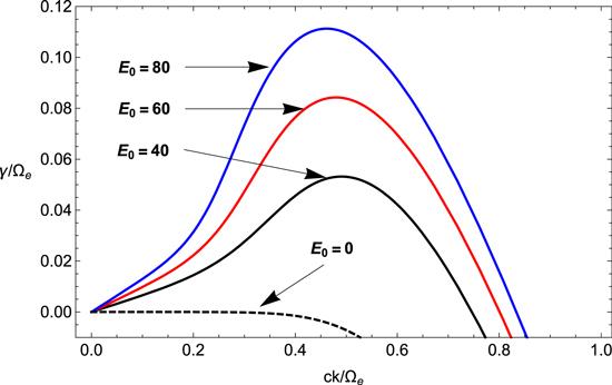
Figure 1. Normalized growth rate versus normalized wave number for different values of ${E}_{o}$ = 0, 40 60, 80 mV m−1 and ${v}_{0}/c$ = 0 with other parameters ${n}_{e}/n$ = 0.9, $\beta =0.15,$ ${\theta }_{\parallel }/c={\theta }_{\perp }/c=0.1,$ ${\omega }_{pe}/{{\rm{\Omega }}}_{e}=0.8$ and $\kappa =4.$ |
In figure 2, growth rate $\gamma /{{\rm{\Omega }}}_{e}$ is plotted against the wave number $ck/{{\rm{\Omega }}}_{e}$ for different values of ${E}_{o}$ = 0 (black), 20 (blue), 40 (red), 80 (orange) in mV m−1 when $\tfrac{{n}_{e}}{n}=0.9,{v}_{0}/c\,=\,0.25\,,{\omega }_{{\rm{pe}}}/{{\rm{\Omega }}}_{e}=0.8,$ $\kappa =5,$ ${\theta }_{\parallel }/c={\theta }_{\perp }/c=0.1$ and $\beta =0.2.$ In figure 2, enhancement of growth rate with the increase in the value of parallel electric field at low values of wave number is evident. We can also note that the range of wave number for which instability occurs also increases with increments in the value of ${E}_{o}.$ Figure 3 is plotted for normalized growth rate $\gamma /{{\rm{\Omega }}}_{e}$ against the normalized wave number $ck/{{\rm{\Omega }}}_{e}$ for different values of $\kappa $ = 4 (black), 5 (blue), 7 (red), 9 (green) when ${E}_{o}=10\,{\rm{mV}}\,{m}^{-1},$ ${n}_{e}/n$ = 0.9, ${\theta }_{\parallel }/c={\theta }_{\perp }/c=0.1,$ ${v}_{0}/c$ = 0.24, ${\omega }_{{\rm{pe}}}/{{\rm{\Omega }}}_{e}=0.8$ and $\beta =0.1.$ We can see that there is an enhancement in the growth rate with the increase in the kappa value. We can also note that the range of wave number for which instability occurs also increases with the increase in the kappa.
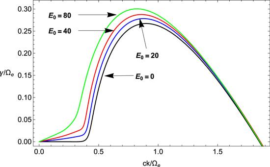
Figure 2. Normalized growth rate versus normalized wave number for different values of electric field ${E}_{o}$ = 0 (black), 20 (blue), 40 (red), 80 (orange) mV m−1 where ${\omega }_{pe}/{{\rm{\Omega }}}_{e}=0.8,$ $\kappa =5,$ ${n}_{e}/n$ = 0.9, ${\theta }_{\parallel }/c={\theta }_{\perp }/c=0.1,$ ${v}_{0}/c$ = 0.25 and $\beta =0.2.$ |
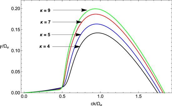
Figure 3. Normalized growth rate versus normalized wave number for different values of electric field $\kappa \,$ = 4 (black), 5 (blue), 7 (red), 9 (green) where ${\omega }_{pe}/{{\rm{\Omega }}}_{e}=0.8,$ ${E}_{o}=10\,\mathrm{mV}/{\rm{m}},$ ${n}_{e}/n$ = 0.9, ${\theta }_{\parallel }/c={\theta }_{\perp }/c=0.1,$ ${v}_{0}/c$ = 0.24 and $\beta =0.1.$ |
The variation in maximum growth rate $\gamma /{{\rm{\Omega }}}_{e}$ against normalized plasma frequency ${\omega }_{{\rm{pe}}}/{{\rm{\Omega }}}_{e}$ has been shown in figure 4 for different values of ${E}_{o}$ = 0, 10, 20, 30, 40 mV m−1 and ${\theta }_{\parallel }/c={\theta }_{\perp }/c=0.1,$ ${n}_{e}/n$ = 0.7, ${v}_{0}/c$ = 0.2, , $\kappa =2.$ In figure 4, it can be seen that when we increase the normalized plasma frequency for a fixed value of ${E}_{o},$ the maximum growth rate increases initially, but after reaching a certain value growth becomes constant for further increase in the plasma frequency. Moreover, we can see that if we fix the value of plasma frequency and increase the value of electric field, the growth rate also increases.
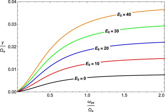
Figure 4. Normalized growth rate versus normalized plasma frequency ${\omega }_{pe}/{{\rm{\Omega }}}_{e}$ for various values of ${E}_{o}$ = 0, 10, 20, 30, 40 mV m−1 with other parameters ${n}_{e}/n$ = 0.7, ${v}_{0}/c$ = 0.2, ${\theta }_{\parallel }/c={\theta }_{\perp }/c=0.1,$ ${\omega }_{pe}/{{\rm{\Omega }}}_{e}=0.8$ and $\kappa =2.$ |
Figure 5 shows the plots for maximum growth rate $(\gamma /{{\rm{\Omega }}}_{e})$ against the trapped electron drift speed ${v}_{0}/c$ for various values of ${E}_{o}$ = 20, 40 60, 80 mV m−1 and for fixed values of $\tfrac{{n}_{e}}{n}=0.9,$ $\beta =0.1,$ ${\omega }_{{\rm{pe}}}/{{\rm{\Omega }}}_{e}=0.8,$ $\kappa =5$ and ${\theta }_{\parallel }/c={\theta }_{\perp }/c=0.1.$ It can be seen that the effect of parallel electric field on the maximum growth rate is more pronounced at the smaller values of trapped electron speed. When we increase the drift speed, maximum growth remains constant initially but it remains higher for larger values of electric field for a fixed value of drift speed. We can also note that there is almost no effect of drift speed on the maximum growth until it reaches a certain threshold value. After reaching that threshold value, trapped electron drift speed dominates the instability and the effect of electric field on the instability reduces, but maximum growth rate increases at a much faster rate with the increase in the drift speed beyond the threshold.
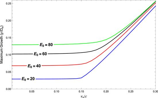
Figure 5. Maximum growth rate versus normalized trapped electron speed for various values of ${E}_{o}$ = 0, 40 60, 80 mV m−1 and ${n}_{e}/n$ = 0.9, $\beta =0.1,$ ${\omega }_{pe}/{{\rm{\Omega }}}_{e}=0.8,$ ${\theta }_{\parallel }/c={\theta }_{\perp }/c=0.1,$ $\kappa =5.$ |
Figure 6 illustrates the variation in maximum growth rate $(\gamma /{{\rm{\Omega }}}_{e})$ versus normalized energetic trapped electron density for different values of ${E}_{o}$ = 20, 40 60, 80 mV m−1, while the other parameters are $\kappa =4,$ ${\omega }_{{\rm{pe}}}/{{\rm{\Omega }}}_{e}=0.8,$ $\beta =0.1,$ ${v}_{0}/c$ = 0.25, ${\theta }_{\parallel }/c={\theta }_{\perp }/c=0.1.$ From figure 6, it can be noted that the maximum growth rate increases with the increase in energetic trapped electron density, but remains higher for larger values of electric field for the fixed value of trapped electron density. Figure 7 is plotted for maximum growth rate $(\gamma /{{\rm{\Omega }}}_{e})$ versus temperature anisotropy $(\tfrac{{T}_{\perp }}{{T}_{\parallel }})$ for different values of ${E}_{o}$ = 20, 40 60, 80 mV m−1 with fixed parameters ${n}_{e}/n$ = 0.9, $\kappa =4,$ $\beta =0.1,$ ${\theta }_{\parallel }/c={\theta }_{\perp }/c=0.1,$ ${\omega }_{pe}/{{\rm{\Omega }}}_{e}=0.8.$ From figure 7, we can note that when we increase temperature anisotropy, maximum growth remains constant initially but is kept higher for larger values of electric field. We can also note that there is almost no effect of trapped electron drift speed on the maximum growth until it reaches a certain threshold value, which is more pronounced for smaller values of electric field. After reaching that threshold value, temperature anisotropy dominates the instability and the effect of electric field on the instability reduces. Furthermore, it is also noted that beyond the threshold when we increase the temperature anisotropy the maximum growth rate increases significantly.
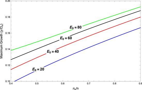
Figure 6. Maximum growth rate versus normalized energetic trapped electron density for different values of ${E}_{o}$ = 20, 40 60, 80 mV m−1 and $\beta =0.1,$ ${v}_{0}/c$ = 0.25, ${\omega }_{pe}/{{\rm{\Omega }}}_{e}=0.8,$ $\kappa =4,$ ${\theta }_{\parallel }/c={\theta }_{\perp }/c=0.1.$ |
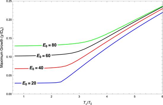
Figure 7. Maximum growth rate versus temperature anisotropy for different values of ${E}_{o}$ = 20, 40 60, 80 mV m−1 with ${n}_{e}/n$ = 0.9, ${\theta }_{\parallel }/c={\theta }_{\perp }/c=0.1,$ ${\omega }_{pe}/{{\rm{\Omega }}}_{e}=0.8,$ $\beta =0.1$ and $\kappa =4.$ |
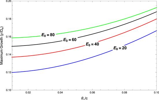
Figure 8 gives the variation in maximum growth rate $(\gamma /{{\rm{\Omega }}}_{e})$ versus perpendicular thermal velocity for various values of ${E}_{o}$ = 20, 40 60, 80 mV m−1 with other parameters ${n}_{e}/n$ = 0.9, ${\theta }_{\parallel }/c=0.1,$ $\beta =0.1,$ ${v}_{0}/c$ = 0.25, ${\omega }_{{\rm{pe}}}/{{\rm{\Omega }}}_{e}\,=0.8$ and $\kappa =4.$ The curves given in figure 8 reveal that when we increase the perpendicular thermal velocity, the maximum growth rate increases monotonically; however, if we fix the value of perpendicular thermal velocity, growth rate shows higher values for a larger electric field.
Figure 8. Maximum growth rate versus ${\theta }_{\perp }/c$ for different values of ${E}_{o}$ = 20, 40, 60, 80 mV m−1 with ${n}_{e}/n$ = 0.9, ${\theta }_{\parallel }/c=0.1,$ $\beta =0.1,$ ${v}_{0}/c$ = 0.25, ${\omega }_{pe}/{{\rm{\Omega }}}_{e}=0.8$ and $\kappa =4.$ |
4. Summary and conclusion
In this paper, the influence of parallel electric field and trapped electron speed and their interplay have been investigated by employing kappa-Maxwellian distribution for auroral trapped electrons on the propagation characteristics of EMEC waves. The general dispersion relation in terms of modified dispersion function ${Z}_{\kappa {\rm{M}}}\left(\xi \right)$ bearing the effects of parallel electric field and trapped electron speed has been derived for the first time by employing kappa-Maxwellian distribution function. The analytical expressions for real frequency and growth rate are then derived and the full dispersion relation is investigated numerically. It is well known that in a drifting plasma the EMEC wave only grows when electron drift speed has values larger than a certain threshold value [39]. However, in the present case our numerical results show that the EMEC wave grows well before the drift speed reaches a threshold value, and has a significant growth rate even for smaller values of parallel electric field. After the drift speed surpasses the threshold value, it dominates the EMEC instability and there is a significant increase in the growth rate. It is concluded that the parallel electric field has a stimulating effect on the growth rate at smaller values of wave number. It is also found that the presence of the electric field provides another source for free energy, and growth can be obtained even in the absence of trapped electron speed and for very small values of temperature anisotropy. In the present study the values of plasma-$\beta $ and the ratio ${\omega }_{{\rm{pe}}}/{{\rm{\Omega }}}_{e}$ have been chosen so that they correspond to a wide range of auroral altitude (Fennell et al 1981). Moreover, with the increase in plasma frequency and perpendicular thermal velocity, the growth rate also increases, but it remains higher for larger values of electric field for the same values of plasma frequency and perpendicular thermal velocity. Thus the present study reveals the interplay of parallel electric field and trapped electron speed on the excitation of EMEC waves in the auroral region.