


1. Introduction
In the year 1998, type Ia Supernova observation [1, 2] revealed the accelerated expansion of the Universe. To explain the observed accelerated expansion of the Universe, the idea of dark energy has been introduced. One of the remarkable features of dark energy is its negative pressure which results in the negative equation of state (ωde). The observed cosmic acceleration is possible only for ωde < −1/3. The cosmological constant is one of the potential candidates of the dark energy bearing equation of state ωλ =−1. The cosmological constant in the constant dark energy model suffers two serious issues namely the coincidence problem and cosmological constant problem. To resolve these two open problems interacting dark energy model has been proposed by a number of authors [3-24] by considering the dynamical behavior of dark energy.
In the interacting dark energy models, transfer of energy between the dominant components of the Universe (matter, dark energy, radiation) is considered. The interaction term Q in the interacting dark energy model concern the transfer of energy between the dominant components of the Universe. One of the major challenges in the interacting dark energy model is to fix the exact functional form of coupling term Q. Different functional forms of coupling term have been used over the years [3-10, 12].
In the absence of a fundamental theory of dark sector physics, the choice of coupling strength in interacting dark energy model might be purely phenomenological. One of the motivations to fix the form of coupling term comes from the dimensional argumentativeness applied to the continuity equation of energy for the components of the Universe. The form of coupling strength can be either the linear function of energy density and the Hubble parameter of the field or the function of the first time derivative of energy density.
In this article, we have discussed the scaling solution of energy density for the two dominant interacting components of the Universe. One component is the scalar field φ which we take as a candidate of dynamical dark energy and the other is dust matter. These two components are interacting via the transfer of their energy into each other. Further, we have estimated the age of the Universe and its variation with the varying coupling constant.
2. Background theory and motivation
In this section, we present a brief introduction to the working background theory of interacting dark energy model. The FLWR metric for flat (K=0) Universe given as
$\begin{eqnarray}{\rm{d}}{s}^{2}=-{\rm{d}}{t}^{2}+{a}^{2}\left(t\right){\left({\rm{d}}{x}^{i}\right)}^{2},\end{eqnarray}$
where a(t) is the expansion scale factor and i=1, 2, 3 represents the spatial component of spacetime. The Friedman equation can be obtained by solving the Einstein field equation for the above metric $\begin{eqnarray}{H}^{2}=\displaystyle \frac{8\pi G}{3}({\rho }_{m}+{\rho }_{{\rm{de}}}),\end{eqnarray}$
where ρm, ρde are energy density of dust matter and dark energy respectively. We are considering a dynamical dark energy model. Although cosmological constant is a potential candidate of constant dark energy, we assume the scalar field as a candidate for dynamical dark energy. A number of scalar fields (quintessence, phantom, tachyonic, etc) have been introduced in physics in different contexts. We scrutinize the dynamical behavior of the tachyonic scalar field (TSF) in the interacting dark energy model by assuming it as one of the candidates for dynamical dark energy.The Lagrangian of TSF appears in string theory in the formulation of tachyon condensate [25-27] given as3 ), the T00 component gives the energy density while the T11 component leads to pressure for the TSF, i.e.
$\begin{eqnarray*}{ \mathcal L }=-V\left(\phi \right)\sqrt{1-{\partial }^{\mu }\phi {\partial }_{\mu }\phi },\end{eqnarray*}$
where V(φ) is the potential of the field. The equation of motion for the spatially homogeneous TSF can be written as $\begin{eqnarray*}\displaystyle \frac{\ddot{\phi }}{1-\dot{{\phi }^{2}}}+3H\dot{\phi }+\displaystyle \frac{V^{\prime} (\phi )}{V(\phi )}=0,\end{eqnarray*}$
and the energy-momentum tensor is $\begin{eqnarray}{T}^{\mu \nu }=\displaystyle \frac{\partial { \mathcal L }}{\partial \left({\partial }_{\mu }\phi \right)}{\partial }^{\nu }\phi -{g}^{\mu \nu }{ \mathcal L }.\end{eqnarray}$
From the energy-momentum tensor equation ( $\begin{eqnarray*}\rho =\displaystyle \frac{V\left(\phi \right)}{\sqrt{1-{\partial }^{\mu }\phi {\partial }_{\mu }\phi }},\end{eqnarray*}$
and $\begin{eqnarray*}p=-V\left(\phi \right)\sqrt{1-{\partial }^{\mu }\phi {\partial }_{\mu }\phi }.\end{eqnarray*}$
For the spatially homogeneous TSF, the energy density and the pressure reduces to the following form $\begin{eqnarray*}\rho =\displaystyle \frac{V\left(\phi \right)}{\sqrt{1-\dot{{\phi }^{2}}}},\ \ \ p=-V\left(\phi \right)\sqrt{1-\dot{{\phi }^{2}}}.\end{eqnarray*}$
3. Interaction between the components
We consider the two dominant components of the Universe are spatially homogeneous TSF (as a candidate of dynamical dark energy) and the dust matter. These two components interact via the transfer of energy. The continuity equation leads to conservation of energy for the two-components. For non-interacting case as, we have4 ). Thus, it is natural that the coupling parameter Q should be a function of energy density and Hubble parameter or the rate of change of energy density of components. Based on phenomenological motivation, several authors [28-32] proposed different forms of interaction term in the interacting dark energy model.
$\begin{eqnarray*}{\dot{\rho }}_{\phi }+3H\left(1+{\omega }_{\phi }\right){\rho }_{\phi }=0,\end{eqnarray*}$
and $\begin{eqnarray*}{\dot{\rho }}_{m}+3H\left(1+{\omega }_{m}\right){\rho }_{m}=0,\end{eqnarray*}$
where wφ=pφ/ρφ. Here wφ, wm is the equation of state parameter for the scalar field φ and the dust matter respectively. During the interaction, individual components can violate the energy conservation but the total energy is conserved. Thus, the energy conservation with the interaction term Q can be represented by the following equations $\begin{eqnarray}\begin{array}{rcl} & & {\dot{\rho }}_{\phi }+3H\left(1+{\omega }_{\phi }\right){\rho }_{\phi }=-Q,\\ & & {\dot{\rho }}_{m}+3H\left(1+{\omega }_{m}\right){\rho }_{m}=Q.\end{array}\end{eqnarray}$
In the absence of the fundamental theory of the dark sector, there are some possible linear and nonlinear functional forms of interaction term Q. One can fix the functional form of Q purely based upon the phenomenological argument which is it should be dimensionally compatible with the left-hand side of equation (In our model we considered a specific functional form of coupling term which is linearly proportional to Hubble parameter H as well as the energy density ρφ of the TSF. This form of coupling term has been used in the literature [33]. Thus we have the following form for interaction term4 ) for given interaction strength equation (5 ) to obtain the following scaling solution of the energy density of components [34]
$\begin{eqnarray}Q=\alpha H{\rho }_{\phi },\end{eqnarray}$
where α is the proportionality constant. One can solve equation ( $\begin{eqnarray*}\displaystyle \frac{{\rho }_{\phi }}{{\rho }_{\phi }^{0}}={\left(\displaystyle \frac{a}{{a}_{0}}\right)}^{-\beta },\end{eqnarray*}$
and $\begin{eqnarray*}\begin{array}{l}\displaystyle \frac{{\rho }_{m}}{{\rho }_{m}^{0}}={\left(\displaystyle \frac{a}{{a}_{0}}\right)}^{-3\left(1+{\omega }_{m}\right)}+\displaystyle \frac{\beta {\rho }_{\phi }^{0}}{{\rho }_{m}^{0}\left[\beta -3\left(1+{\omega }_{m}\right)\right]}\\ \quad \times \ \left[{\left(\displaystyle \frac{a}{{a}_{0}}\right)}^{-3\left(1+{\omega }_{m}\right)}-{\left(\displaystyle \frac{a}{{a}_{0}}\right)}^{-\beta }\right],\end{array}\end{eqnarray*}$
where β=α + 3(1 + ωφ), ${\rho }_{\phi }^{0}$ (${\rho }_{m}^{0}$) is the present value of scalar field (dust matter), and a0 is the present value of scale factor. If $\dot{\phi }\to 0$, i.e. for constant φ we get ρφ → ρλ (someconstant). In this approximation limit TSF mimics the cosmological constant, and we have β=α. Hence, the scaling solution reduces to the following form $\begin{eqnarray}\displaystyle \frac{{\rho }_{\lambda }}{{\rho }_{\lambda }^{0}}={\left(\displaystyle \frac{a}{{a}_{0}}\right)}^{-\alpha },\end{eqnarray}$
$\begin{eqnarray}\begin{array}{l}\displaystyle \frac{{\rho }_{m}}{{\rho }_{m}^{0}}={\left(\displaystyle \frac{a}{{a}_{0}}\right)}^{-3\left(1+{\omega }_{m}\right)}+\displaystyle \frac{\alpha {\rho }_{\lambda }^{0}}{{\rho }_{m}^{0}\left[\alpha -3\left(1+{\omega }_{m}\right)\right]}\\ \quad \times \ \left[{\left(\displaystyle \frac{a}{{a}_{0}}\right)}^{-3\left(1+{\omega }_{m}\right)}-{\left(\displaystyle \frac{a}{{a}_{0}}\right)}^{-\alpha }\right].\end{array}\end{eqnarray}$
4. Functional form of scale factor
In this section, we investigate the evolution of the expansion scale factor (a) for the two important cases. The interaction proportionality constant term (α) can be either zero or non-zero. So, we are considering the following two case
4.1. For α=0
From the Friedmann equations (equation (2 )) along with the scaling solutions equations (6 ) and (7 ), we have8 ) gives9 ), we get the analytical expression for x as a function of cosmic time t
$\begin{eqnarray}H=\sqrt{\displaystyle \frac{8\pi G}{3}}\sqrt{{\rho }_{\lambda }^{0}+{\rho }_{m}^{0}{x}^{-3(1+{\omega }_{m})}},\end{eqnarray}$
where $x=\displaystyle \frac{a}{{a}_{0}}$, a0 is the present value scale factor. Equation ( $\begin{eqnarray}{\rm{d}}t=\displaystyle \frac{A{\rm{d}}x}{x\sqrt{1+{B}^{2}{x}^{-3(1+{\omega }_{m})}}},\end{eqnarray}$
where $\begin{eqnarray*}A=\sqrt{\displaystyle \frac{3}{k{\rho }_{\lambda }^{0}}},\,\,B=\sqrt{\displaystyle \frac{{\rho }_{m}^{0}}{{\rho }_{\lambda }^{0}}},\ \ \,\mathrm{and}\,\,k=8\pi G.\end{eqnarray*}$
Solving equation ( $\begin{eqnarray}x={\left[{B}^{-2}{\left(\tanh \left(\displaystyle \frac{3(1+{\omega }_{m})t}{2A}\right)\right)}^{2}-{B}^{-2}\right]}^{-\tfrac{1}{3(1+{\omega }_{m})}}.\end{eqnarray}$
4.2. For α ≠ 0
In this case, equation (8 ) leads to the following equation11 ) to obtain an expression of t in terms of x, we have12 ) can be rewritten as13 )), we have n=1, $\alpha ^{\prime} =0$, $A^{\prime} =A$ and, $B^{\prime} =B$. Hence, the term inside the bracket of equations (14 ) can be written as15 ) and equation (14 ) we get14 ) reduces to the same form which we will obtain by integrating the equation (9 ).
$\begin{eqnarray}{\rm{d}}t=\displaystyle \frac{A^{\prime} {\rm{d}}x}{{x}^{\left(1-\tfrac{\alpha }{2}\right)}\sqrt{1+B{{\prime} }^{2}{x}^{\alpha -3(1+{\omega }_{m})}}},\end{eqnarray}$
where $\begin{eqnarray*}\begin{array}{rcl}A^{\prime} & = & \sqrt{\displaystyle \frac{3(1+{\omega }_{m})-\alpha }{k{\rho }_{\lambda }^{0}(1+{\omega }_{m})}},\\ {\rm{and}}\,\,B^{\prime} & = & \sqrt{\displaystyle \frac{3(1+{\omega }_{m}){\rho }_{m}^{0}-\alpha ({\rho }_{\lambda }^{0}+{\rho }_{m}^{0})}{3(1+{\omega }_{m}){\rho }_{\lambda }^{0}}}.\end{array}\end{eqnarray*}$
Solving equation ( $\begin{eqnarray}\begin{array}{rcl}t & = & \displaystyle \frac{2A^{\prime} }{{\left(-1\right)}^{n}B{{\prime} }^{\alpha ^{\prime} }[\alpha -3(1+{\omega }_{m})]}\left[{\sqrt{1+B{{\prime} }^{2}{x}^{\alpha -3(1+{\omega }_{m})}}}_{2}{{F}}_{1}\right.\\ & & \left.\times \left(\displaystyle \frac{1}{2},n,\displaystyle \frac{3}{2},{\left(\sqrt{1+B{{\prime} }^{2}{x}^{\alpha -3(1+{\omega }_{m})}}\right)}^{2}\right)\right],\end{array}\end{eqnarray}$
where $\begin{eqnarray}\alpha ^{\prime} =\displaystyle \frac{\alpha }{\alpha -3(1+{\omega }_{m})},\ \ n=\displaystyle \frac{\tfrac{\alpha }{2}-3(1+{\omega }_{m})}{\alpha -3(1+{\omega }_{m})}.\end{eqnarray}$
The function 2F1 hypergeometric functional series defined by [35] $\begin{eqnarray*}{}_{2}{{F}}_{1}(a,b,c,z)=\displaystyle \sum _{m=0}^{\infty }\displaystyle \frac{{\left(a\right)}_{m}{\left(b\right)}_{m}}{{\left(c\right)}_{m}}\displaystyle \frac{{z}^{m}}{m!},\end{eqnarray*}$
where $\begin{eqnarray*}{\left(a\right)}_{m}=\left\{\begin{array}{ll}1 & \,m=0,\\ a(a+1)..(a+m-1) & \,m\gt 0.\end{array}\right.\end{eqnarray*}$
By using the definition of 2F1, equation ( $\begin{eqnarray}\begin{array}{rcl}t & = & \displaystyle \frac{2A^{\prime} }{{\left(-1\right)}^{n}B{{\prime} }^{\alpha ^{\prime} }\left[\alpha -3(1+{\omega }_{m})\right]}\left(\Space{0ex}{3.6ex}{0ex}\sqrt{1+B{{\prime} }^{2}{x}^{\alpha -3(1+{\omega }_{m})}}\right.\\ & & +\displaystyle \frac{1}{3}n\displaystyle \frac{{\left(\sqrt{1+B{{\prime} }^{2}{x}^{\alpha -3(1+{\omega }_{m})}}\right)}^{3}}{1!}\\ & & +\left.\displaystyle \frac{1}{5}n(n+1)\displaystyle \frac{{\left(\sqrt{1+B{{\prime} }^{2}{x}^{\alpha -3(1+{\omega }_{m})}}\right)}^{5}}{2!}+...\right).\end{array}\end{eqnarray}$
When α=0 (from equations ( $\begin{eqnarray}\begin{array}{l}{\tanh }^{-1}\sqrt{1\,+\,{B}^{2}{x}^{-3(1+{\omega }_{m})}}=\sqrt{1\,+\,{B}^{2}{x}^{-3(1+{\omega }_{m})}}\\ \quad +\,\displaystyle \frac{1}{3}{\left(\sqrt{1+{B}^{2}{x}^{-3(1+{\omega }_{m})}}\right)}^{3},\\ \quad +\,\displaystyle \frac{1}{5}{\left(\sqrt{1+{B}^{2}{x}^{-3(1+{\omega }_{m})}}\right)}^{5}+....\end{array}\end{eqnarray}$
Using equation ( $\begin{eqnarray}t=\displaystyle \frac{2A}{3(1+{\omega }_{m})}{\tanh }^{-1}\sqrt{1+{B}^{2}{x}^{-3(1+{\omega }_{m})}}.\end{eqnarray}$
In the limit α → 0, equation (5. Age of the Universe (AoU)
The age of the Universe has been discussed in the [14] by considering two-phase (interacting and non-interacting dark energy) evolution of the Universe. Recent data [36] provide the present value of Hubble parameter H0 to be approximately 67.66 ± 0.42 km s−1 Mpc−1 and the present value of normalized energy density parameters are ${{\rm{\Omega }}}_{\lambda }^{0}=0.6889\pm 0.0056$, ${{\rm{\Omega }}}_{m}^{0}=0.3111\pm 0.0056$. In this section, we estimate the age of the Universe with and without coupling between the matter and the TSF (candidate of dynamical dark energy).
5.1. Without interaction (α=0)
One can find the cosmic age in the absence of interaction by integrating the equation (9 ) to get
$\begin{eqnarray*}{t}_{a}={\int }_{0}^{1}\displaystyle \frac{A{\rm{d}}x}{x\sqrt{1+{B}^{2}{x}^{-3(1+{\omega }_{m})}}}.\end{eqnarray*}$
For the Hubble constant H0=67.66 km s−1 Mpc−1, energy density parameter ${{\rm{\Omega }}}_{\lambda }^{0}=0.6889$, and ${{\rm{\Omega }}}_{m}^{0}=0.3111$, we found the age of the Universe to be ${t}_{a}\approx 0.9543{H}_{0}^{-1}\approx 13.52\,\mathrm{Gyr}$. The value of ${H}_{0}^{-1}$ is ≈ 14.167 Gyr.5.2. With interaction (α ≠ 0)
In presence of interaction the age of the Universe can be derived from equation (11 ) and it comes out be [37]2 ), (6 ), and equation (7 ) for ωm=0, we have17 ) gives
$\begin{eqnarray*}{t}_{a}(x)={\int }_{0}^{x}\displaystyle \frac{{\rm{d}}x^{\prime} }{x^{\prime} H(x^{\prime} )},\end{eqnarray*}$
which can be modified as $\begin{eqnarray}{t}_{a}(x){H}_{0}={\int }_{0}^{x}\displaystyle \frac{{\rm{d}}x^{\prime} }{x^{\prime} E(x^{\prime} )},\end{eqnarray}$
where $E(x)=\displaystyle \frac{H(x)}{{H}_{0}}$ and, $x=\displaystyle \frac{a}{{a}_{0}}$. Using equations ( $\begin{eqnarray*}E(x)=\sqrt{\left({{\rm{\Omega }}}_{m}^{0}+\displaystyle \frac{\alpha }{\alpha -3}{{\rm{\Omega }}}_{\lambda }^{0}\right){x}^{-3}-{{\rm{\Omega }}}_{\lambda }^{0}\left(\displaystyle \frac{3}{\alpha -3}\right){x}^{-\alpha }}.\end{eqnarray*}$
Thus the equation ( $\begin{eqnarray}{t}_{a}(x){H}_{0}={\int }_{0}^{1}\displaystyle \frac{{\rm{d}}x^{\prime} }{\sqrt{\left({{\rm{\Omega }}}_{m}^{0}+\tfrac{\alpha }{\alpha -3}{{\rm{\Omega }}}_{\lambda }^{0}\right){\left(x^{\prime} \right)}^{-1}-{{\rm{\Omega }}}_{\lambda }^{0}\left(\tfrac{3}{\alpha -3}\right){\left(x^{\prime} \right)}^{2-\alpha }}}.\end{eqnarray}$
The cosmic age of Universe in the presence of coupling α for its various numerical values is (from α=0 to α=0.9) given in the table 1 for ${{\rm{\Omega }}}_{\lambda }^{0}=0.7$, ${{\rm{\Omega }}}_{m}^{0}=0.3$ and, ${{\rm{\Omega }}}_{\lambda }^{0}\,=0.6889$, ${{\rm{\Omega }}}_{m}^{0}=0.3111$.6. Variation of Ωλ, Ωm with ${\rm{ln}}\,a$
Here we have observed the variation of energy density parameter Ωλ and Ωm as a function of $\eta =\mathrm{ln}\,a$ by following the method of [38]. We can define two new variable ${ \mathcal X }$ and ${ \mathcal Y }$ such that ${ \mathcal X }=\displaystyle \frac{8\pi G}{3{H}^{2}}{\rho }_{\lambda }={{\rm{\Omega }}}_{\lambda }$, and ${ \mathcal Y }=\displaystyle \frac{8\pi G}{3{H}^{2}}{\rho }_{m}={{\rm{\Omega }}}_{m}$. Differentiating ${ \mathcal X }$ and ${ \mathcal Y }$ with η, we have4 ), we get2 ) we get21 ), (22 ) in equations (19 ), equation (20 ), we get the following set of equations
$\begin{eqnarray}\displaystyle \frac{{\rm{d}}{ \mathcal X }}{{\rm{d}}\eta }=\displaystyle \frac{1}{H}\left[\displaystyle \frac{8\pi G}{3{H}^{2}}{\dot{\rho }}_{\lambda }-2\displaystyle \frac{8\pi G}{3{H}^{3}}{\rho }_{\lambda }\dot{H}\right],\end{eqnarray}$
$\begin{eqnarray}\displaystyle \frac{{\rm{d}}{ \mathcal Y }}{{\rm{d}}\eta }=\displaystyle \frac{1}{H}\left[\displaystyle \frac{8\pi G}{3{H}^{2}}{\dot{\rho }}_{m}-2\displaystyle \frac{8\pi G}{3{H}^{3}}{\rho }_{m}\dot{H}\right].\end{eqnarray}$
From equations ( $\begin{eqnarray}{\dot{\rho }}_{\lambda }=-\alpha H{\rho }_{\lambda },\ \ \ \ \ \ {\dot{\rho }}_{m}=\alpha H{\rho }_{\lambda }-3H{\rho }_{m},\end{eqnarray}$
and from equations ( $\begin{eqnarray}\displaystyle \frac{\dot{H}}{{H}^{2}}=-\displaystyle \frac{3}{2}\displaystyle \frac{8\pi G}{3{H}^{2}}{\rho }_{m},\ \ \ \ \ \ { \mathcal X }+{ \mathcal Y }=1.\end{eqnarray}$
So using, equations ( $\begin{eqnarray}\displaystyle \frac{{\rm{d}}{ \mathcal X }}{{\rm{d}}\eta }+3{{ \mathcal X }}^{2}+(\alpha -3){ \mathcal X }=0,\end{eqnarray}$
$\begin{eqnarray}\displaystyle \frac{{\rm{d}}{ \mathcal Y }}{{\rm{d}}\eta }-3{{ \mathcal Y }}^{2}+(\alpha +3){ \mathcal Y }-\alpha =0.\end{eqnarray}$
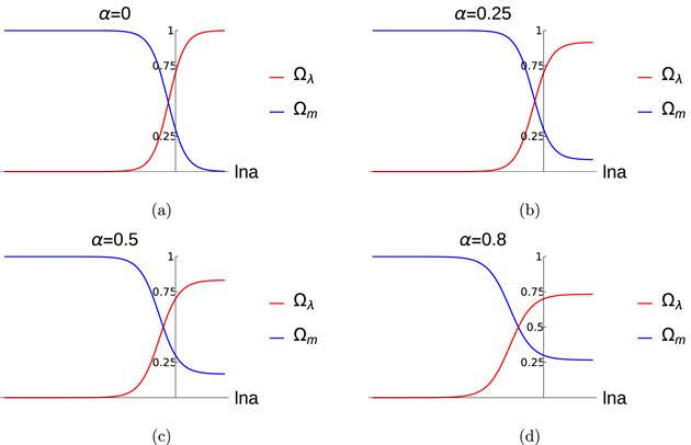
Figure 1. Plots of Ωλ and Ωm as a function of $\eta (=\mathrm{ln}\,a)$ for different values coupling parameter α. The vertical axis represents the present cosmological time. |
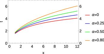
Figure 2. Graphical variation of equations ( |
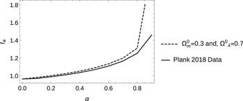
Figure 3. Graphical variation of table 1. Here we observe the evolution of age of the Universe with the coupling constant α. |
Table 1. Age of Universe (AOU) ta for different values of coupling constant α. First table (left one) is for ${{\rm{\Omega }}}_{\lambda }^{0}=0.7,\,{{\rm{\Omega }}}_{m}^{0}=0.3$ and second one (right one) is for ${{\rm{\Omega }}}_{\lambda }^{0}=0.6889$, ${{\rm{\Omega }}}_{m}^{0}=0.3111$. |
| α | AOU in terms of ${H}_{0}^{-1}$ | α | AOU in terms of ${H}_{0}^{-1}$ | |
|---|---|---|---|---|
| 0 | 0.964 | 0 | 0.964 | |
| 0.1 | 0.981 | 0.1 | 0.970 | |
| 0.2 | 1.001 | 0.2 | 0.989 | |
| 0.3 | 1.024 | 0.3 | 1.010 | |
| 0.4 | 1.052 | 0.4 | 1.036 | |
| 0.5 | 1.088 | 0.5 | 1.068 | |
| 0.6 | 1.134 | 0.6 | 1.109 | |
| 0.7 | 1.199 | 0.7 | 1.166 | |
| 0.8 | 1.311 | 0.8 | 1.254 | |
| 0.9 | 2.222 | 0.9 | 1.459 |
7. Conclusion
In this article we studied the evolution of scale factor by considering the two interacting components (matter and dark energy) in the spatially flat Universe. We considered the spatially homogeneous TSF as a candidate of dark energy. In the interacting dark energy model, the two components are mutually coupled via coupling parameter Q, and a transfer of energy between the two components is possible. During the interaction, the individual components can violate the energy conservation, but overall energy is conserved. In the absence of a fundamental theory of dark sector the choice of coupling parameter is purely phenomenological. We obtained the age of the Universe in interacting dark energy model and presented in table 1 for different value of coupling constant. We found that with the increase in the value of coupling constant (α), the age of the Universe is also increasing. But as we further increased the value of coupling constant (beyond 1), the age of the Universe turns out to be imaginary which is a non-physical situation. This puts an upper bound to the coupling constant α, and it should be less than 1. We plotted the normalized energy density of dark energy (Ωλ) and matter (Ωm) as a function of $\mathrm{ln}\,a$ in figure 1. Figure 2 showed the relationship between the cosmic time and the normalized dimensionless scale factor x. And in figure 3, we plotted the data of table 1 which shows the variation of the age of the Universe with the coupling constant α.