


1. Introduction
Nonlinear evolution equations (NLEEs) can model various nonlinear phenomena that occur in nature and science, which has attracted extensive attention of many research groups around the world. The exact solutions of NLEEs have been put on the agenda for a better understanding of those nonlinear phenomena, and a series of mature techniques have been proposed, such as the Hirota bilinear method [1–6], the Darboux transformation [7–11], the inverse scattering transformation [12–14], the Lie group analysis [15] and other techniques [16–19]. Specially, the most representative one is the celebrated Korteweg–de Vries (KdV) equation [20].
$\begin{eqnarray}{U}_{t}+6{{UU}}_{x}++{U}_{{xxx}}=0.\end{eqnarray}$
This equation was first written by Korteweg and De Vries in 1895, and demonstrated the possibility of solitary wave generation. The KdV equation has been derived from plasma physics [21, 22], hydrodynamics, anharmonic (nonlinear) lattices [23, 24] and other physical settings, and its generalized versions are frequently used to describe many physical phenomena in many physical systems. Potential Kadomtsev–Petviashvili (PKP) equation that came as a natural generalization of the KdV equation can be read as follows [12, 25–35] $\begin{eqnarray}{u}_{{xt}}+\alpha {u}_{x}{u}_{{xx}}+\beta {u}_{{xxxx}}+\gamma {u}_{{yy}}=0,\qquad \end{eqnarray}$
α, β and γ are arbitrary real constants. This equation describes the dynamics of small and finite amplitude waves in (2 + 1)-dimension. It is also generated in certain physical contexts assuming that the wave is moving along x and that all changes in y are slower than in the direction of motion [12]. Pohjanpelto described the variational double complex of the PKP equation by the invariant form under symmetric algebra, and computed the cohomology of the relevant Euler–Lagrangian complex [25]; The local conservation laws and infinite symmetry group of the PKP equation are surveyed by Rosenhaus [26]; The nonlocal symmetries and interaction solutions of the PKP equation are derived by Ren Bo through truncated Painlev $\acute{e}$ analysis [27]; Senthilvelon [28], Kaya [29] and Zhang [30] obtained the kink soliton solutions; Kumar [31] studied the closed-form solutions such as multiple-front wave, kink wave and curve-shaped multisoliton; Xian [32] and Dai [33] investigated the breather solutions; Luo developed the first-order lump solution of the PKP equation by using a homoclinic test technique [34, 35]. But high-order breather, M-lump and semi-rational solutions of PKP equation have never been reported.Motivated by the above considerations and the value of the PKP equation in physical systems, we focus on the high-order breather, M-lump and semi-rational solutions of PKP equation, The structure of this paper is organized as follows. In section 2 , we obtain the N-soliton and high-order breather solutions by means of the Hirota method and exhibit the limit process of high-order breathers. In section 3 , M-lumps are generated by taking the long wave limit of obtained solitons. In section 4 , the semi-rational solutions with elastic collision are generated by taking a long-wave limit and the main results of the paper are summarized in section 5 .
2. N-soliton and high-order breather solutions of PKP equation
For a start, through the following dependent variable transformation2 ) produces the following bilinear form
$\begin{eqnarray}u=\displaystyle \frac{12\beta }{\alpha }{\partial }_{x}\mathrm{ln}f(x,y,t).\end{eqnarray}$
The PKP equation ( $\begin{eqnarray*}[{D}_{x}{D}_{t}+\beta {D}_{x}^{4}+\gamma {D}_{y}^{2}]f(x,y,t)\cdot f(x,y,t)=0,\end{eqnarray*}$
here f is a real function and D is the Hirota’s bilinear differential operator [1]. Then, the N soliton solutions u can be generated using the bilinear method [1], in which f is written as follows: $\begin{eqnarray}f=\displaystyle \sum _{\mu =0,1}\exp \left(\displaystyle \sum _{j\lt k}^{(N)}{\mu }_{j}{\mu }_{k}{A}_{{jk}}+\displaystyle \sum _{j=1}^{N}{\mu }_{j}{\eta }_{j}\right).\end{eqnarray}$
Here $\begin{eqnarray}\begin{array}{l}\exp \left({A}_{{jk}}\right)\\ \ =\ \displaystyle \frac{\left\{\begin{array}{c}({p}_{j}^{5}{p}_{k}+{p}_{j}{q}_{k}^{5})(\beta -\alpha )+(4\alpha -\beta )({p}_{j}^{2}{p}_{k}^{4}+{p}_{j}^{4}{p}^{2})\\ -\gamma {\left({p}_{j}{q}_{k}-{q}_{j}{p}_{k}\right)}^{2}-6\alpha {p}_{j}^{2}{p}_{k}^{3}\end{array}\right\}}{3\beta {p}_{j}^{2}{p}_{k}^{2}{\left({p}_{j}+{p}_{k}\right)}^{2}-\gamma {\left({p}_{j}{q}_{k}-{q}_{j}{p}_{k}\right)}^{2}},\\ {\eta }_{j}={p}_{j}x+{q}_{j}y+{{\rm{\Omega }}}_{j}t+{\eta }_{j}^{0},\\ {{\rm{\Omega }}}_{j}=-\displaystyle \frac{\gamma {q}_{j}^{2}}{{p}_{j}^{2}}-\beta {p}_{j}^{3},\end{array}\,\end{eqnarray}$
where pj, qj are arbitrary real parameters, ${\eta }_{j}^{0}$ is a complex constant, and the subscript j denotes an integer. The notation ∑μ=0 indicates summation over all possible combinations of μ1 = 0, 1, μ2 = 0, 1, ⋯ , μn = 0, 1. The ${\sum }_{j\lt k}^{(N)}$ summation is over all possible combinations of the N elements in the specific condition of j < k. In this paper, we set the parameter γ = − 1 for all specific examples and figures.In order to obtained the n-order breather solutions of the PKP equation, the following parametric restrictions must be held in equation (4 )6 ), and its analytic expression is as follows:
$\begin{eqnarray}N=2n,\quad {p}_{j}^{* }={p}_{j+n},\quad {q}_{j}^{* }={q}_{j+n},\quad {\eta }_{j}^{0}={\eta }_{n+j}^{0},\end{eqnarray}$
first-order breather solution ${u}_{1\mathrm{bre}}$ is obtained with parameters α = 1, β = 1, γ = − 1, p1 = ib, ${\eta }_{1}^{0}=0$ and q1 = c in equation ( $\begin{eqnarray}\begin{array}{l}{u}_{1\mathrm{bre}}\\ \ =\ \displaystyle \frac{24{{bc}}^{2}[\cosh ({cy})+\sinh ({cy})]\sin ({b}^{3}t+{bx}-\tfrac{{c}^{2}}{b}t)}{2{c}^{2}\left\{\begin{array}{c}[\cosh ({cy})+\sinh ({cy})]\cos ({b}^{3}t+{bx}-\tfrac{{c}^{2}}{b}t)\\ \quad \ +\ (3{b}^{4}+{c}^{2})[\cosh (2{cy})+\sinh (2{cy})]\end{array}\right\}+{c}^{2}}.\end{array}\end{eqnarray}$
From the above expressions, it is obvious that the period of the first-order breather solution is controlled by the parameter b, the smaller the value of ∣b∣, the greater the period of the first-order breather solution, as is shown in figure 1 where panel (e) is the corresponding two-dimensional plot of the panel (d).
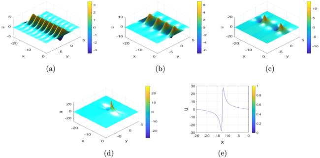
Figure 1. First-order breather solution ${u}_{1\mathrm{bre}}$ for the PKP equation with parameter c = 1 at t = 0, (a): b = 2; (b): b = 1; (c): b = $\tfrac{1}{2};$ (d): b = $\tfrac{1}{4};$ (e): y = 0, b = $\tfrac{1}{4}$. |
Second-order breather solutions of synchronization period are obtained with parameters α = 1, β = 1, γ = − 1, p1 = ib, p3 = ib, ${\eta }_{1}^{0}=0$, ${\eta }_{3}^{0}=0$, q1 = a and q3 = c in equation (6 ), then the functions f can be rewritten as
$\begin{eqnarray}\begin{array}{rcl}f & = & \displaystyle \frac{2}{{A}_{11}}[\cosh ({B}_{11})+\sinh ({B}_{11})]\cos ({B}_{21})\\ & & +\ \displaystyle \frac{6{A}_{12}{C}_{11}}{{c}^{2}{A}_{11}}[\cosh ({B}_{12})\\ & & +\ \sinh ({B}_{12})]\cos ({B}_{22})+2[\cosh ({B}_{13})\\ & & +\ \sinh ({B}_{13})]\cos ({B}_{22})\\ & & +\ \displaystyle \frac{2{A}_{12}{C}_{12}}{{a}^{2}{A}_{11}}[\cosh ({B}_{14})+\sinh ({B}_{14})]\\ & & \times \ \cos ({B}_{23})+2[\cosh ({B}_{15})\\ & & +\ \sinh ({B}_{15})]\cos ({B}_{23})+\displaystyle \frac{24{b}^{4}}{{\left(a+c\right)}^{2}}\\ & & \times \ [\cosh ({B}_{11})+\sinh ({B}_{11})]\cos ({B}_{24})\\ & & +\ 2[\cosh ({B}_{11})+\sinh ({B}_{11})]\cos ({B}_{24})\\ & & +\ \displaystyle \frac{3{C}_{11}{C}_{12}{A}_{12}^{2}}{{a}^{2}{c}^{2}{A}_{11}^{2}}[\cosh (2{B}_{11})\\ & & +\ \sinh (2{B}_{11})]+\displaystyle \frac{{C}_{12}}{{a}^{2}}[\cosh (2{B}_{13})\\ & & +\ \sinh (2{B}_{13})]+\displaystyle \frac{3{C}_{11}}{{c}^{2}}[\cosh (2{B}_{15})\\ & & +\ \sinh (2{B}_{15})]+1,\end{array}\end{eqnarray}$
where
$\begin{eqnarray*}\begin{array}{rcl}{A}_{11} & = & {\left(a+c\right)}^{2}[12{b}^{4}+{\left(a-c\right)}^{2}],\\ {A}_{12} & = & {\left(a-c\right)}^{2}[12{b}^{4}+{\left(a+c\right)}^{2}],\\ {B}_{11} & = & (a+c)y,\quad {B}_{12}=(a+2c)y-1,\quad {B}_{13}={ay}+1,\\ {B}_{14} & = & (2a+c)y+1,\quad {B}_{15}={cy}-1,\\ {B}_{21} & = & -2{bx}-2{b}^{3}t+\displaystyle \frac{{a}^{2}+{c}^{2}}{b}t,\\ {B}_{22} & = & {bx}-{b}^{3}t-\displaystyle \frac{{c}^{2}}{b}t,\quad {B}_{23}={bx}+{b}^{3}t-\displaystyle \frac{{c}^{2}}{b}t,\\ {B}_{24} & = & \displaystyle \frac{{a}^{2}-{c}^{2}}{b}t,{C}_{11}={b}^{4}+\displaystyle \frac{1}{3}{c}^{2},\ {C}_{12}={a}^{2}+3{b}^{2}.\end{array}\end{eqnarray*}$
The second-order breather solutions are generated by the superposition of two identical period of breather through selecting above special parameters see (figure 2). Where panel (f) is the corresponding two-dimensional plot of the panel (e). Additionally, third-order breather solutions of synchronization period are also acquired with parameters α = 1, β = 1, γ = − 1, p1 = ib, p3 = ib, p5 = ib, ${\eta }_{1}^{0}=\tfrac{\pi }{3}$, ${\eta }_{3}^{0}=6\pi $, ${\eta }_{5}^{0}=-\pi $, ${q}_{1}=\tfrac{1}{2}$, q3 = 1 and ${q}_{5}=\tfrac{1}{3}$ in (6 ). They have the same period because of the same value of pj (j = 1, 2, 3, 4, 5, 6), see figure 3.

Figure 2. Second-order breather solutions for the PKP equation with parameters a = $\tfrac{1}{2}$ and c = $\tfrac{1}{3}$ at t = 0, (a): b = $\tfrac{3}{2};$ (b): b = 1; (c): b = $\tfrac{1}{2};$ (d): b = $\tfrac{1}{3};$ (e): b = $\tfrac{1}{5};$ (f): x = 0, b = $\tfrac{1}{5}$. |
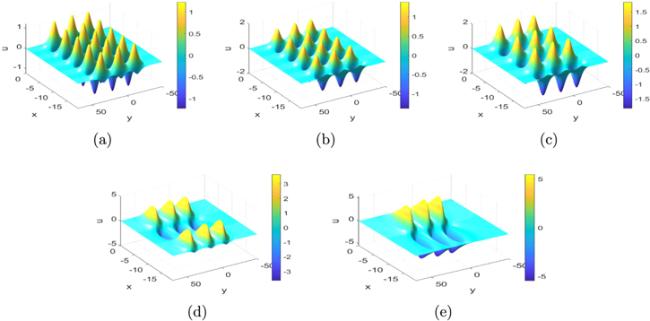
Figure 3. Third-order breather solutions for the PKP equation at t = 0, (a): b = $\tfrac{3}{2};$ (b): b = $\tfrac{4}{3};$ (c): b = 1; (d): b = $\tfrac{1}{2};$ (e): b = $\tfrac{1}{3}$. |
3. M-lump solutions of PKP equation
In this section, we focus on the lump solutions of equation (2 ), to construct the M-lump solutions in the (x, y)-plane, we have to take the parameters in equation (4 )4 ) becomes a polynomial function
$\begin{eqnarray}{N}=2n,\ {q}_{{j}}={\lambda }_{{j}}{{p}}_{{j}},\ {\eta }_{{j}}^{0}={\rm{i}}\pi \ (1\leqslant {j}\leqslant {N}),\end{eqnarray}$
and take a limit as pj → 0. Then the function f defined in equation ( $\begin{eqnarray}\begin{array}{l}f={f}_{N}=\displaystyle \prod _{k=1}^{N}{\theta }_{k}+\displaystyle \frac{1}{2}\displaystyle \sum _{k,j}^{(N)}{\alpha }_{{kj}}\displaystyle \prod _{l\ne k,j}^{N}{\theta }_{l}+\cdots +\displaystyle \frac{1}{M!{2}^{M}}\\ \ \times \ \displaystyle \sum _{i,j,\ldots ,m,n}^{(N)}\mathop{\overbrace{{\alpha }_{{kj}}{\alpha }_{{kl}}\cdots {\alpha }_{{mn}}}}\limits^{M}\displaystyle \prod _{p\ne k,j,\ldots m,n}^{N}{\theta }_{p}+\cdots ,\end{array}\end{eqnarray}$
with $\begin{eqnarray}{\theta }_{j}=x+{\lambda }_{j}-\gamma {\lambda }_{j}^{2}t,\ {\alpha }_{{jk}}=\displaystyle \frac{12\beta }{\gamma {\left({\lambda }_{j}-{\lambda }_{k}\right)}^{2}}.\end{eqnarray}$
Here k and j are positive integers. We must emphasize that λj is a complex constant and ${\lambda }_{j}^{* }={\lambda }_{n+j}$. By virtue of transformation $u=\tfrac{12\beta }{\alpha }{\partial }_{x}\mathrm{ln}f(x,y,t)$, the rational solution of PKP equation can be obtained. This process can be proved by a similar way in [36].3.1. 2-lump solution
1-lump solution can be generated in the (x, y)-plane by taking N = 2, λ1 = a + ib and λ2 = a − ib in equation (10 ), and corresponding solution is given explicitly by the following formula
$\begin{eqnarray}u=\displaystyle \frac{x+{ay}+24{b}^{2}({a}^{2}-{b}^{2})t}{\left\{\begin{array}{c}3+{\left({a}^{2}b+{b}^{3}\right)}^{2}{\left(\tfrac{{a}^{2}-{b}^{2}}{{a}^{2}+{b}^{2}}x+\tfrac{a}{{a}^{2}+{b}^{2}}y+t\right)}^{2}\\ +\tfrac{{b}^{4}}{{\left({a}^{2}+{b}^{2}\right)}^{2}}{\left(2{ax}+({a}^{2}+{b}^{2})y\right)}^{2}\end{array}\right\}}.\end{eqnarray}$
From the above expression we can see that the lump solution is smooth. Figure 4(a) is the three-dimensional plot of the 1-lump solution with parameters a = 0 and b = 4. Figure 4(b) is the corresponding two-dimensional plot of the figure 4(a). The dynamic behavior of the 1-lump is similar to the lump that appears in the [34, 35].

Figure 4. 1-lump (a) and 2-lump (c) for the PKP equation at t = 0. Panel (b) is the cross sectional profile of (a) along y = 0; panel (d) is the cross sectional profile of (c) along x = − 15. |
3.2. 3-lump solution
Furthermore, 2-lump solution are generated with parameters N = 4, ${\lambda }_{1}=\tfrac{5i}{2}$ and ${\lambda }_{3}=\tfrac{5i}{5}$ in equation (10 ), in which f can be written as follows:3 ). Figure 4(c) is the three-dimensional plot of 2-lump, figure 4(d) is the corresponding two-dimensional plot of the figure 4(c).
$\begin{eqnarray}\begin{array}{rcl}f & = & {\theta }_{1}\,{\theta }_{2}\,{\theta }_{3}\,{\theta }_{4}+{a}_{12}\,{\theta }_{3}\,{\theta }_{4}+{a}_{13}\,{\theta }_{2}\,{\theta }_{4}\\ & & +\ {a}_{14}\,{\theta }_{2}\,{\theta }_{3}+{a}_{23}\,{\theta }_{1}{\theta }_{4}+{a}_{24}\,{\theta }_{1}\,{\theta }_{3}\\ & & +\ {a}_{34}\,{\theta }_{1}\,{\theta }_{2}+{a}_{12}\,{a}_{34}+{a}_{13}\,{a}_{24}+{a}_{14}\,{a}_{23}\\ & = & \ {x}^{4}-\displaystyle \frac{325}{18}{{tx}}^{3}+\left[\displaystyle \frac{325}{36}{y}^{2}+\displaystyle \frac{150625}{1296}{t}^{2}\right.\\ & & +\ \left.\displaystyle \frac{23439}{625}\right]{x}^{2}-\left[\displaystyle \frac{203125}{648}{t}^{3}+\displaystyle \frac{625}{9}{{ty}}^{2}+\displaystyle \frac{51097}{150}t\right]x\\ & & +\ \displaystyle \frac{625}{36}{y}^{4}+\left(\displaystyle \frac{203125}{1296}{t}^{2}-\displaystyle \frac{39047}{300}\right){y}^{2}\\ & & +\ \displaystyle \frac{390625}{1296}{t}^{4}+\displaystyle \frac{289393}{432}{t}^{2}+\displaystyle \frac{117029124}{390625},\end{array}\end{eqnarray}$
which yields the 2-lump of the PKP equation by means of equation (3.3. 3-lump solution
Additional, we also derive the 3-lump solution u given by equation (3 ), taking
$\begin{eqnarray}N=6,M=3,{\eta }_{{j}}^{0}={\rm{i}}\pi \quad (1\leqslant {j}\leqslant 6),\end{eqnarray}$
in (
$\begin{eqnarray}\begin{array}{rcl}f & = & {\theta }_{1}\,{\theta }_{2}\,{\theta }_{3}\,{\theta }_{4}\,{\theta }_{5}\,{\theta }_{6}+{a}_{12}\,{\theta }_{3}\,{\theta }_{4}\,{\theta }_{5}\,{\theta }_{6}\\ & & +\ {a}_{13}\,{\theta }_{2}\,{\theta }_{4}\,{\theta }_{5}\,{\theta }_{6}+{a}_{14}\,{\theta }_{2}\,{\theta }_{3}\,{\theta }_{5}\,{\theta }_{6}\\ & & +\ {a}_{15}\,{\theta }_{2}\,{\theta }_{3}\,{\theta }_{4}\,{\theta }_{6}+{a}_{16}\,{\theta }_{2}\,{\theta }_{3}\,{\theta }_{4}\,{\theta }_{5}\\ & & +\ {a}_{23}\,{\theta }_{1}\,{\theta }_{4}\,{\theta }_{5}\,{\theta }_{6}+{a}_{24}\,{\theta }_{1}\,{\theta }_{3}\,{\theta }_{5}\,{\theta }_{6}\\ & & +\ {a}_{25}\,{\theta }_{1}\,{\theta }_{3}\,{\theta }_{4}\,{\theta }_{6}+{a}_{26}\,{\theta }_{1}\,{\theta }_{3}\,{\theta }_{4}\,{\theta }_{5}\\ & & +\ {a}_{34}\,{\theta }_{1}\,{\theta }_{2}\,{\theta }_{5}\,{\theta }_{6}+{a}_{35}\,{\theta }_{1}\,{\theta }_{2}\,{\theta }_{4}\,{\theta }_{6}\\ & & +\ {a}_{36}\,{\theta }_{1}\,{\theta }_{2}\,{\theta }_{4}\,{\theta }_{5}+{a}_{45}\,{\theta }_{1}\,{\theta }_{2}\,{\theta }_{3}\,{\theta }_{6}\\ & & +\ {a}_{46}\,{\theta }_{1}\,{\theta }_{2}\,\theta 3\,{\theta }_{5}+{a}_{56}\,{\theta }_{1}\,{\theta }_{2}\,{\theta }_{3}\,{\theta }_{4}\\ & & +\ {a}_{12}\,{a}_{34}\,{\theta }_{5}\,{\theta }_{6}+{a}_{12}\,{a}_{35}\,{\theta }_{4}\,{\theta }_{6}\\ & & +\ {a}_{12}\,{a}_{36}\,{\theta }_{4}\,{\theta }_{5}+{a}_{12}\,{a}_{45}\,{\theta }_{3}\,{\theta }_{6}\\ & & +\ {a}_{12}\,{a}_{46}\,{\theta }_{3}\,{\theta }_{5}+{a}_{12}\,{a}_{56}\,{\theta }_{3}\,{\theta }_{4}\\ & & +\ {a}_{13}\,{a}_{24}\,{\theta }_{5}\,{\theta }_{6}+{a}_{13}\,{a}_{25}\,{\theta }_{4}\,{\theta }_{6}\\ & & +\ {a}_{13}\,{a}_{26}\,{\theta }_{4}\,{\theta }_{5}+{a}_{13}\,{a}_{45}\,{\theta }_{2}\,{\theta }_{6}\\ & & +\ {a}_{13}\,{a}_{46}\,{\theta }_{2}\,{\theta }_{5}+{a}_{13}\,{a}_{56}\,{\theta }_{2}\,{\theta }_{4}\\ & & +\ {a}_{14}\,{a}_{23}\,{\theta }_{5}\,{\theta }_{6}+{a}_{14}\,{a}_{25}\,{\theta }_{3}\,{\theta }_{6}\\ & & +\ {a}_{14}\,{a}_{26}\,{\theta }_{3}\,{\theta }_{5}+{a}_{14}\,{a}_{35}\,{\theta }_{2}\,{\theta }_{6}\\ & & +\ {a}_{14}\,{a}_{36}\,{\theta }_{2}\,{\theta }_{5}+{a}_{14}\,{a}_{56}\,{\theta }_{2}\,{\theta }_{3}\\ & & +\ {a}_{15}\,{a}_{23}\,{\theta }_{4}\,{\theta }_{6}+{a}_{15}\,{a}_{24}\,{\theta }_{3}\,{\theta }_{6}\\ & & +\ {a}_{15}\,{a}_{26}\,{\theta }_{3}\,{\theta }_{4}+{a}_{15}\,{a}_{34}\,{\theta }_{2}\,{\theta }_{6}\\ & & +\ {a}_{15}\,{a}_{36}\,{\theta }_{2}\,{\theta }_{4}+{a}_{15}\,{a}_{46}\,{\theta }_{2}\,{\theta }_{3}\\ & & +\ {a}_{16}\,{a}_{23}\,{\theta }_{4}\,{\theta }_{5}+{a}_{16}\,{a}_{24}\,{\theta }_{3}\,{\theta }_{5}\\ & & +\ {a}_{16}\,{a}_{25}\,{\theta }_{3}\,{\theta }_{4}+{a}_{16}\,{a}_{34}\,{\theta }_{2}\,{\theta }_{5}\\ & & +\ {a}_{16}\,{a}_{35}\,{\theta }_{2}\,{\theta }_{4}+{a}_{16}\,{a}_{45}\,{\theta }_{2}\,{\theta }_{3}\\ & & +\ {a}_{23}\,{a}_{45}\,{\theta }_{1}\,{\theta }_{6}+{a}_{23}\,{a}_{46}\,{\theta }_{1}\,{\theta }_{5}\\ & & +\ {a}_{23}\,{a}_{56}\,{\theta }_{1}\,{\theta }_{4}+{a}_{24}\,{a}_{35}\,{\theta }_{1}\,{\theta }_{6}\\ & & +\ {a}_{24}\,{a}_{36}\,{\theta }_{1}\,{\theta }_{5}+{a}_{24}\,{a}_{56}\,{\theta }_{1}\,{\theta }_{3}\\ & & +\ {a}_{25}\,{a}_{34}\,{\theta }_{1}\,{\theta }_{6}+{a}_{25}\,{a}_{36}\,{\theta }_{1}\,{\theta }_{4}\\ & & +\ {a}_{25}\,{a}_{46}\,{\theta }_{1}\,{\theta }_{3}+{a}_{26}\,{a}_{34}\,{\theta }_{1}\,{\theta }_{5}\\ & & +\ {a}_{26}\,{a}_{35}\,{\theta }_{1}\,{\theta }_{4}+{a}_{26}\,{a}_{45}\,{\theta }_{1}\,{\theta }_{3}\\ & & +\ {a}_{34}\,{a}_{56}\,{\theta }_{1}\,{\theta }_{2}+{a}_{35}\,{a}_{46}\,{\theta }_{1}\,{\theta }_{2}\\ & & +\ {a}_{36}\,{a}_{45}\,{\theta }_{1}\,{\theta }_{2}+{a}_{12}\,{a}_{34}\,{a}_{56}\\ & & +\ {a}_{12}\,{a}_{35}\,{a}_{46}+{a}_{12}\,{a}_{36}\,{a}_{45}\\ & & +\ {a}_{13}\,{a}_{24}\,{a}_{56}+{a}_{13}\,{a}_{25}\,{a}_{46}\\ & & +\ {a}_{13}\,{a}_{26}\,{a}_{45}+{a}_{14}\,{a}_{23}\,{a}_{56}\\ & & +\ {a}_{14}\,{a}_{25}\,{a}_{36}+{a}_{14}\,{a}_{26}\,{a}_{35}\\ & & +\ {a}_{15}\,{a}_{23}\,{a}_{46}+{a}_{15}\,{a}_{24}\,{a}_{36}\\ & & +\ {a}_{15}\,{a}_{26}\,{a}_{34}+{a}_{16}\,{a}_{23}\,{a}_{45}\\ & & +\ {a}_{16}\,{a}_{24}\,{a}_{35}+{a}_{16}\,{a}_{25}\,{a}_{34},\end{array}\end{eqnarray}$
where
$\begin{eqnarray}{\theta }_{j}=x+{\lambda }_{j}-\gamma {\lambda }_{j}^{2}t,\quad {a}_{{jk}}=\displaystyle \frac{12\beta }{\gamma {\left({\lambda }_{j}-{\lambda }_{k}\right)}^{2}}.\end{eqnarray}$
Further, we take ${\lambda }_{1}=\tfrac{7{\rm{i}}}{10}$, ${\lambda }_{3}=\tfrac{9{\rm{i}}}{10}$ and ${\lambda }_{5}=\tfrac{4{\rm{i}}}{5}$, 3-lump wave solution are generated, see figure 5.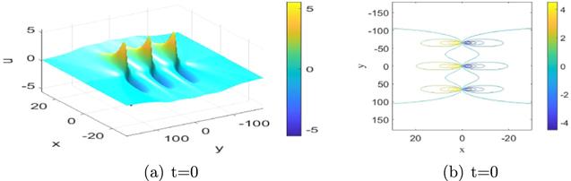
Figure 5. 3-lump solution for the PKP equation; panel (b) is the contour plot of (a). |
4. Semi-rational solutions of PKP equation
In this section, we mainly concentrate on the semi-rational solution of PKP equation (2 ). The semi-rational solutions may be generated by taking a long-wave limit of only a part of exponential functions in f. Setting4 ) become a combination of polynomial and exponential functions, which generate semi-rational solutions u of PKP equation (2 ).
$\begin{eqnarray}1\lt 2j\lt N,\quad 1\leqslant k\leqslant 2j,\quad {q}_{k}={\lambda }_{k}{p}_{k},\quad {\eta }_{k}^{0}={\rm{i}}\pi ,\end{eqnarray}$
then taking the limit pk → 0 for all k, the functions f defined in equation (4.1. A hybrid solution between 1-lump and 1-soliton
We first consider the case of N = 3. Setting4 ), we obtain11 ) and (5 ). Further, we take λ1 = 1 + i, λ1 = 1 − i, p3 = 1, q3 = − 1 and ${\eta }_{3}^{0}=0$ in equation (19 ). The analytic expression of the semi-rational solution uls is as follows
$\begin{eqnarray}\begin{array}{rcl}N & = & 3,{q}_{1}={\lambda }_{1}{p}_{1},{q}_{2}={\lambda }_{2}{p}_{2},{\eta }_{1}^{0}={\eta }_{2}^{0}={\rm{i}}\pi ,\\ \alpha & = & 1,\beta =1,\gamma =-1,\end{array}\end{eqnarray}$
and taking p1, p2 → 0 in equation ( $\begin{eqnarray}\begin{array}{rcl}f & = & ({\theta }_{1}{\theta }_{2}+{a}_{12})+({\theta }_{1}{\theta }_{2}+{a}_{12}+{a}_{13}{\theta }_{2}\\ & & +\ {a}_{23}{\theta }_{1}+{a}_{12}{a}_{23}){e}^{{\eta }_{3}},\end{array}\end{eqnarray}$
where ${a}_{j3}=\tfrac{-12{p}_{3}^{3}}{{({q}_{3}-{\lambda }_{j}{p}_{3})}^{2}+3{p}_{3}^{4}}$ and θj, a12, η3 are given by equations ( $\begin{eqnarray}\begin{array}{l}{u}_{{ls}}=\displaystyle \frac{\left\{\begin{array}{c}\left[312{\left(y+t+\tfrac{1}{2}x+\tfrac{7}{26}\right)}^{2}+312{\left(t-\tfrac{1}{2}x+\tfrac{7}{26}\right)}^{2}+312\right]{e}^{x-y}\\ \qquad \ +\ 312(x+y)\end{array}\right\}}{\left\{\begin{array}{c}\left[26{\left(y+t+\tfrac{1}{2}x-\tfrac{3}{13}\right)}^{2}+\tfrac{13}{2}{\left(x-2t-\tfrac{30}{13}\right)}^{2}+39\right]{e}^{x-y}\\ \quad \ +13{\left(x+y\right)}^{2}+52{\left(t+\tfrac{1}{2}y\right)}^{2}+39\end{array}\right\}}.\end{array}\end{eqnarray}$
The corresponding semi-rational solution uls describes the interaction between a lump and a kink soliton. As seen in figure 6, with the evolution of time, the velocities and amplitudes of the kink soliton and the lump have not changed before and after the collision.
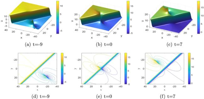
Figure 6. The time evolution in the (x, y)-plane of the semi-rational solution uls. Panels (a)–(c) are the contour plots of (d)–(f) respectively. |
4.2. A hybrid solution between 1-lump and 2-soliton
For larger N, the semi-rational solution consisting of a lump and more solitons will be generated with appropriate parameters. For example4 ), we obtain
$\begin{eqnarray}\begin{array}{rcl}N & = & 4,{q}_{1}={\lambda }_{1}{p}_{1},{q}_{2}={\lambda }_{2}{p}_{2},{\eta }_{1}^{0}={\eta }_{2}^{0}={\rm{i}}\pi ,\\ \alpha & = & 1,\beta =1,\gamma =-1,\end{array}\end{eqnarray}$
and taking p1, p2 → 0 in equation ( $\begin{eqnarray}\begin{array}{rcl}f & = & {e}^{{A}_{34}}({a}_{13}{a}_{23}+{a}_{13}{a}_{24}+{a}_{13}{\theta }_{2}+{a}_{14}{a}_{23}\\ & & +\ {a}_{14}{a}_{24}+{a}_{14}{\theta }_{2}\\ & & +\ {a}_{23}{\theta }_{1}+{a}_{24}{\theta }_{1}+{\theta }_{1}{\theta }_{2}+{a}_{12}){e}^{{\eta }_{3}+{\eta }_{4}}\\ & & +\ ({a}_{13}{a}_{23}+{a}_{13}{\theta }_{2}\\ & & +\ {a}_{23}{\theta }_{1}+{\theta }_{1}{\theta }_{2}+{a}_{12}){e}^{{\eta }_{3}}\\ & & +\ ({a}_{14}{a}_{24}+{a}_{14}{\theta }_{2}+{a}_{24}{\theta }_{1}+{\theta }_{1}{\theta }_{2}\\ & & +\ {a}_{12}){e}^{{\eta }_{4}}+{\theta }_{1}{\theta }_{2}+{a}_{12},\end{array}\end{eqnarray}$
where
$\begin{eqnarray*}{a}_{{js}}=\displaystyle \frac{-12{p}_{s}^{3}}{{\left({q}_{s}-{\lambda }_{j}{p}_{s}\right)}^{2}+3{p}_{s}^{4}},j=(1,2),s=(3,4),\end{eqnarray*}$
and θj is defined by equation (22 ). Taking p3, p4, q3 and q4 are real parameters, the semi-rational solution consisting of a lump and two kink solitons is obtained see figure 7. This semi-rational solution is also elastic collision, which is different from the semi-rational solution of inelastic collision in [35].

Figure 7. The time evolution in the (x, y)-plane of the semi-rational solution consisting of a lump and two kink solitons given by equation ( |
4.3. A hybrid solution between 1-lump and 1-breather
Additionally, we take ${p}_{3}={p}_{4}^{* },{q}_{3}^{* }={q}_{4}$ and ${\eta }_{3}^{0}={\eta }_{4}^{0}$ in equation (22 ), a new semi-rational understanding consisting of a lump and a breather is generated see figure 8. To the best of authors knowledge, the obtained semi-rational solutions of equation (2 ) in this section have never been reported before.

Figure 8. Semi-rational solutions u plotted in the (x, y)-plane, consisting of a lump and a breather solutions for equation ( |
5. Discussion and conclusion
In this paper, N-soliton, high-order synchronized breather and M-lump solutions for the PKP equation are presented based on the Hirota method and long wave limit. We give the limit process of the period of the first-order second-order and third-order synchronized breather solutions (see figures 1–3). Through the analysis of exact expressions and plots, it is easy to find that the first-order (see figures 1(d), (e)), second-order (see figures 2(e), (f)) and third-order (see figure 3(e)) synchronized breather solutions are perfectly matched to 1-lump (see figures 4(a), (b)), 2-lump [see figures 4(c), (d)] and 3-lump (see figure 5(a)). Furthermore, the semi-rational solutions of equation (2 ) are obtained by taking the limit of some exponential functions in equation (4 ). Figures 6 and 7 describe the collision between lump and solitons, which is different from the semi-rational solution of inelastic collision in [35]. Additionally, by choosing appropriate parameters, the dynamics of the superposition between a lump and a breather is demonstrated in figure 8.