


1. Introduction
In nuclear physics, the quantum shape-phase transition (QSPT) has received much interest in recent decades [1–12]. QSPTs are abrupt changes within the structure of the energy spectrum, caused by a change in the parameters of the quantum Hamiltonian. With QSPT, the concept critical point [3–8], based on very simple shaped potentials, describes the dynamical symmetry of the nuclear system at points of QSPT between various phases. Up to now, the studies based on these potentials concentrate on the studying of the QSPTs and their critical points, however, during the past three years, a new approach has been proposed for the sake of shape coexistence phenomena and shape fluctuations phenomena [9–12]. This new direction is based on the introduction of a barrier that separates two (or more) configurations of states. By changing the barrier height, one can have coexistence phenomena or fluctuations phenomena. This behavior could be achieved by anharmonic oscillator potentials (AOPs) with sextic anharmonicity. By the separation of variables, these problems are reduced to solve the one-dimensional Schrödinger equation.
Recently [13], we extended these type of results to a two-dimensional space and test the ability of three types of two-dimensional potentials in generating the advantages of the infinite square well potential (ISWP). Actually, the potential for a QSPT at the critical point possesses nearly flat shape. These potentials are characterized by the existence of barriers in its structure and can evolve from a very narrow deformed minimum separated by high barriers to a near flat case, depending on a few parameters. For these potentials, when the tunneling is taken into consideration, the level $E$ splits into four levels, ${E}_{1},$ ${E}_{2},$ ${E}_{3}$ and ${E}_{4},$ i.e. the states appear as closely spaced quartets. We will call this mode of the system tunneling splitting mode (TSM). The quantum tunneling strength among the four minima is determined by the features of the separating barrier. The fluctuations phenomena take place when the wave function peaks begin to combine and join together, but yet distinguishable. This circumstance is obtained when the potentials are symmetric and the tunneling is strong.
In the first part of this work, we shift the analysis from the one that focuses on ISWP and critical points to one that focuses on harmonic oscillator potential (HOP). To this end, first, we introduce three categories of two-dimensional Davidson-like potentials (DLPs) and investigate their ability in reproducing the properties of the HOP and AOPs. They present a transition of spectra from TSM to fluctuations phenomena ending with the spectra of the HOP or AOPs, depending on the height of the barrier. On the contrary, these potentials can evolve from wide spherical minima separated by high barriers to a near flat case or HOP. Moreover, we give an explanation of the coexistence phenomena of two tunneling splitting configurations in two-dimensional space based on these potentials.
On the other hand, the dynamical octupole correlations have attracted special focus because they are the cornerstone in the explanation of many negative parity states like the ${1}^{-}$ states in the spectra of even–even nuclei that are considered as important indicators of the reflection-asymmetric nuclei [14–20]. The main benchmark of whether a nucleus is octupole deformation or not is the existence of the negative-parity band, ${L}^{\pi }={1}^{-},{3}^{-},{5}^{-},\ldots ,$ located nearby the ground-state band and building together a single band with ${L}^{\pi }={0}^{+},{1}^{-},{2}^{+},{3}^{-},{4}^{+},\ldots .$ whilst the positive-and negative-parity bands remain separated from each other, for nuclei in vibration regions. A diversity of methods and techniques were utilized to study the role of the octupole degree of freedom. These include density functional models [21–23], interacting boson and boson vector models [24, 25], and collective models, such as the coherent quadrupole–octupole model (CQOM) [26, 27].
In the second part of this study, using CQOM, the DLPs are used for studying the yrast and non-yrast energy bands with alternating parity in 100Mo, 146,148Nd, 148,150Sm, 220Ra, 220,222Rn, and 220,222Th. We study the physical consequences of the two-dimensional oscillations with respect to the quadrupole ${\beta }_{2}$ and octupole ${\beta }_{3}$ variables. Good agreement has been found between the calculated and measured spectra. A detailed comparison with the predictions of HOP and DLPs is performed. The global parametrization for selected nuclei is achieved. The results of our investigation show that the existence of the barrier is essential in any description of octupole deformed nuclei. Consequently, DLPs provide an extended version of the CQOM which having the ability to reproduce the spectra in even–even quadrupole–octupole shape deformed nuclei.
In section 2 , the fluctuations phenomena and coexistence phenomena in two dimensions are analyzed using three classes of DLPs. Section 3 is devoted to a discussion of the CQOM applications in different regions in the nuclear landscape and the numerical results. Section 4 summarizes the results of our work.
2. Fluctuations and coexistence phenomena in two dimensions
In [13], we studied the energy spectra of three types of AOPs which play an essential role in nuclear structure and exhibited multi-dimensional quantum tunneling. These potentials are
$\begin{eqnarray}{H}_{\alpha }(x,y)={x}^{2\alpha }+{y}^{2\alpha },\end{eqnarray}$
$\begin{eqnarray}{V}_{\alpha }^{(a)}\left(x,y\right)=1/2a-\left({x}^{2}+{y}^{2}\right)+a\left({x}^{2\alpha }+{y}^{2\alpha }\right),\end{eqnarray}$
$\begin{eqnarray}{U}_{\alpha }^{(b,c)}\left(x,y\right)=\left({x}^{2}+{y}^{2}\right)-b\left({x}^{4}+{y}^{4}\right)+c\left({x}^{2\alpha }+{y}^{2\alpha }\right),\end{eqnarray}$
where $a,$ $b$ and $c$ are free parameters and $\alpha =2,3,4.$ The predictions for wave functions and spectra are obtained by using the nine-point finite-difference method (for more details see [13]). It has been demonstrated that the purely AOPs, ${H}_{\alpha },$ provide a ‘bridge’ between the HOP and ISWP. Furthermore, the evolution of energy spectra of the AOPs, ${V}_{\alpha }^{(a)}$ and ${U}_{\alpha }^{(b,c)},$ as a function of barrier height and normalized to the ground state energy, shows that the transition is changed from TSM to fluctuations phenomena passing by the ${H}_{\alpha }$ spectra ending with the spectrum of the ISWP.The AOPs, ${H}_{\alpha },$ ${V}_{\alpha }^{(a)},$ ${U}_{\alpha }^{(b,c)},$ and ISWP are appropriate for the transition between two quantum phases, particularly, if one of the phases is related to HOP and simultaneously offer new features. The ISWP is the most important one because of its simplicity and analytic solvability. The purely AOPs, ${H}_{2},$ ${H}_{3},$ and ${H}_{4},$ change from the HOP to the ISWP, respectively. Here, we focus our attention on the purely AOPs ${H}_{\alpha }$ because their predictions of the spectra do not include free parameters, therefore provide valuable points of reference in the Casten triangle. In nuclear physics, the one-dimensional version of the purely AOPs ${H}_{\alpha }$ are X(5)-${\beta }^{2\alpha }$ and E(5)-${\beta }^{2\alpha }$ models. One might ask: are there other flexible potentials that are able to provide us with the properties of ${H}_{\alpha },$ depending on a very limited number of parameters and are characterized by the presence of barriers in its structure? Of course, these potentials will allow us to model various deformation related features such as critical points, coexistence phenomena, fluctuations phenomena, and QSPT, which appear in the complex dynamics of many nuclei, particularly, quadrupole–octupole shape deformations nuclei.
First, we will consider the DLPs which are chosen to be of the following form:4 ) with regard to the parameter $d$ is shown in figure 1(b). The first part of ${W}_{\alpha }^{(d,e)}$ is ${H}_{\alpha }$ and the second part produces the barrier. Both the barrier height and thickness increase with the increase of $d,$ but decrease when $e$ increase. The curvature of the minima is more spherical than the minima of the AOPs ${V}_{\alpha }^{(a)}.$ We restrict our attention to the region $R=\left\{\left(d,e\right):d,e\in \left[0.1,1\right]\right\},$ where the DLPs (4 ) evolve from four minima (as in figure 1(c)) to the near flat case,${H}_{\alpha },$ (shown in figure 1(d)).
$\begin{eqnarray}{W}_{\alpha }^{(d,e)}\left(x,y\right)=\left({x}^{2\alpha }+{y}^{2\alpha }\right)+\displaystyle \frac{d}{{x}^{2\alpha }+e}+\displaystyle \frac{d}{{y}^{2\alpha }+e},\end{eqnarray}$
where d and e are free parameters and α = 2, 3, …. These potentials can be approached to purely AOPs, ${H}_{\alpha },$ and, at the same time, are characterized by the existence of barriers. The shape of the potential depends on the values of $d$ and $e,$ see figure 1. The DLPs ${W}_{\alpha }^{(d,e)}\left(x,y\right)$ are symmetric about the $x$- and $y$-axis, with a core at the center, $(x,y)=(0,0).$ The evolution of the vertical cross-sections of the DLPs (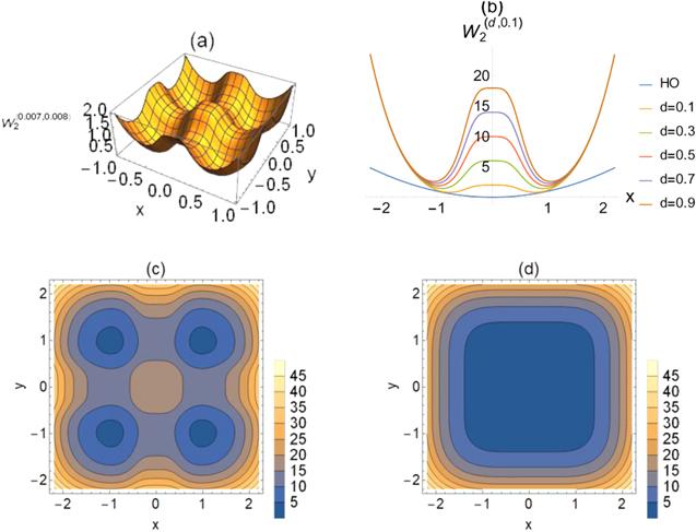
Figure 1. (a) The three-dimensional representation of the DLPs ${W}_{2}^{(0.007,0.008)}\left(x,y\right).$ (b) The vertical cross-sections of the DLPs ${W}_{2}^{(d,0.1)}\left(x,y\right).$ (c) and (d) are the two-dimensional representation of the potentials ${W}_{2}^{(1,0.1)}\left(x,y\right)$ and ${W}_{2}^{(1,1)}\left(x,y\right),$ respectively (contour plots). The potential changes from four minima potential to approximately flat minimum potential, ${H}_{2}.$ (For interpretation of the colors in the figure(s), the reader is referred to the web version of this article.) |
We are now able to investigate the evolution of the spectra of the DLPs ${W}_{\alpha }^{(d,e)}$ as a function of the parameters $d$ and $e.$ It is sufficient and valuable to survey this behavior at the four boundaries of $R.$ The energy spectra of the DLPs, ${W}_{\alpha }^{(0.1,e)}$ and ${W}_{\alpha }^{(1,e)},$ $0.1\leqslant e\leqslant 1$ and $\alpha =2$ are presented in figures 2(a) and (b), respectively. The energy spectrum shows a transition from the spectrum of the TSM to the ${H}_{\alpha }$ solution, figure 2(b). The TSM is achieved for small values of $e,$ where the DLP forms wide spherical minima separated by high barriers. The other limit occurs for high values of $e,$ where the ${H}_{2}$ term is dominant. It is important to stress that we obtained here the TSM from large spherical minima separated by high barriers. However, for the AOPs ${V}_{\alpha }^{(a)}$ or ${U}_{\alpha }^{(b,c)},$ this mode is generated from very narrow deformed minima separated by high barriers. Obviously, the DLPs ${W}_{\alpha }^{(d,e)}$ and the AOPs ${V}_{\alpha }^{(a)}$ or ${U}_{\alpha }^{(b,c)}$ are in two sides of ISWP. Similarly, we can study the evolution of the spectra on the other two boundaries of $R.$ The energy spectra of the DLPs, ${W}_{\alpha }^{(d,0.1)}$ and ${W}_{\alpha }^{(d,1)},$ $0.1\leqslant d\leqslant 1,$ are presented in figures 2(c) and (d), respectively. These potentials have the fourfold TSM for high values of $d,$ but the energy spectra, for small values of $d,$ can be considered very close to the spectra of the ${H}_{\alpha },$ figure 2(c).
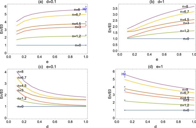
Figure 2. Representation of the first nine energy levels, as a function of $d$ and $e$ for DLPs ${W}_{2}^{(d,e)}\left(x,y\right),$ (normalized to the ground state energy). (a) and (b) show the behavior of the spectra of the DLPs ${W}_{2}^{(d,e)}\left(x,y\right)$ against the parameter $e$ with $d=0.1$ and $1,$ respectively. However, (c) and (d) display the energy spectra of the potential against the parameter $d$ with $e=0.1$ and $1,$ respectively. |
A better understanding of such models is fulfilled by investigating the probability density, ${\left|{\rm{\Psi }}\left(x,y\right)\right|}^{2}.$ The development of the ground state and first excited state wave functions of the DLPs ${W}_{2}^{(1,e)},$ as a function of $e,$ is represented in figure 3. Beginning from $e=0.05,$ the ground state wave function is composed of four separate peaks. At $e=0.1,$ the four peaks of probability density become closely spaced and begin to combine and join together. At $e=0.2,$ the probability density forms an isolated island with four peaks. At $e=0.3,$ the crest of probability density is approximately flat and squared in the shape. When the ground state becomes above the barrier, at $e=\,1,$ we have a normal single-peak probability density for the ground state. In the same manner, at $e=0.05,$ the first excited state wave function is composed of two separate peaks and two separate troughs. By increasing the value of $e,$ the four peaks of the probability density, with unequal height, become closely spaced. At a specific point, the probability density of the first excited state wave function is composed of two pieces. When the first excited state is near the top of the barrier, each piece of probability density is delocalized and more extended over the corresponding two minima and has two unequal peaks, one peak around the first minimum, however, the second peak spreads to the other minimum. At $e=1,$ we have normal two peaks probability density, with equally high, figure 3.
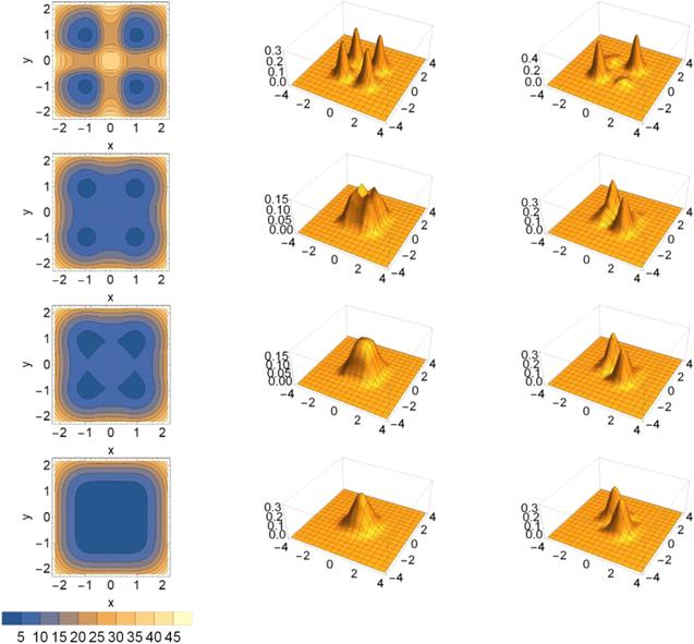
Figure 3. The contour plots of the DLPs ${W}_{2}^{(1,e)}\left(x,y\right)$ (left panel), the ground state probability density (medial panel), and the probability density of first excited state (right panel), as $e=0.05,$ $0.2,$ $0.3,$ and $1$ from top to bottom, obtained numerically. |
These results show the capability of the DLPs, ${W}_{2}^{(d,e)},$ which are characterized by wide spherical minima separated by high barriers, to approach ${H}_{2}.$ As expected, the results, particularly the behavior of the wave functions, are similar to those for the AOPs ${V}_{\alpha }^{(a)}$ or ${U}_{\alpha }^{(b,c)}$ [13] because the parameters are in the region $R,$ where the DLPs (4 ) evolve from four minima to the near flat case, however, in this case, the potentials are on the other side of ISWP.
Additionally, with barrier structure, the following potentials can be approached to HOP5 ) is shown in figure 4(b), as a function of $f.$ The first part of the DLPs (5 ) is the HOP and the second part produces the barrier. The height and thickness of the barrier increase with the increase of $f,$ but decrease with the increase of $g.$ The curvature of the potential is completely inside the HOP. Again, we focus on the region $R=\{\left(f,g\right),f,g\in \left[0.1,1\right]\},$ see figures 4(c) and (d).
$\begin{eqnarray}{Q}_{\alpha }^{\left(f,g\right)}\left(x,y\right)=\left({x}^{2}+{y}^{2}\right)+\displaystyle \frac{f}{{x}^{2\alpha }+g}+\displaystyle \frac{f}{{y}^{2\alpha }+g},\end{eqnarray}$
where $f$ and $g$ are free parameters and $\alpha =2,3,\ldots .$ The shape-changing of the vertical cross-sections of the DLPs (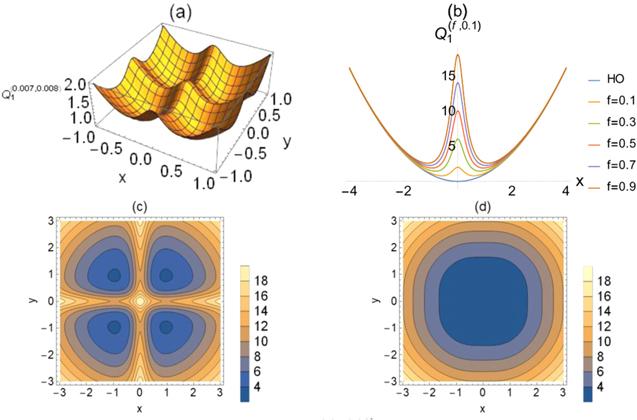
Figure 4. (a) The three-dimensional representation of the DLPs ${Q}_{1}^{(0.07,0.08)}\left(x,y\right).$ (b) The vertical cross-sections of the DLPs ${Q}_{1}^{(f,0.1)}\left(x,y\right).$ (c) and (d) are the contour plots of the potentials ${Q}_{1}^{(1,0.1)}\left(x,y\right)$ and ${Q}_{1}^{(1,1)}\left(x,y\right),$ respectively. The potential changes from four minima potential to HOP, ${H}_{1}.$ |
The energy spectra of the DLPs ${Q}_{\alpha }^{(f,0.1)},$ ${Q}_{\alpha }^{(f,1)},$ ${Q}_{\alpha }^{(0.1,g)}$ and ${Q}_{\alpha }^{(1,g)},$ $0.1\leqslant f\leqslant 1,$ $0.1\leqslant g\leqslant 1$ and $\alpha =2,$ presented in figure 5, show a transition from the spectrum of the HOP solution to the TSM. However, this transition is totally different from the ${W}_{\alpha }^{(d,e)},$ ${U}_{\alpha }^{(b,c)}$ and ${V}_{\alpha }^{(a)}$ cases. The upper level with $n=3,$ from the first quartet of levels, and the lower levels with $n=4,5,$ from the second quartet of levels, evolve such that they form the three-fold degenerate level of HOP, figures 5(b) and (c). Similarly, the upper levels $n=6,7,$ from the second quartet, and the lower level $n=8,$ from the third quartet, are a portion from the four-fold degenerate level of HOP. Actually, the potentials ${W}_{\alpha }^{(d,e)},$ ${U}_{\alpha }^{(b,c)}$ and ${V}_{\alpha }^{(a)}$ evolve from four minima potentials to the near flat case, ${H}_{\alpha }$ or ISWP while the DLPs ${Q}_{\alpha }^{\left(f,g\right)}$ evolve from four minima potentials to HOP.
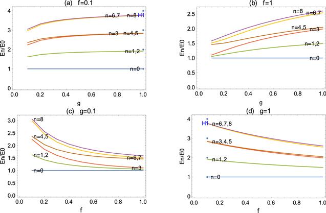
Figure 5. Representation of the first nine energy levels, as a function of $f$ and $g$ for DLPs ${Q}_{1}^{(f,g)}\left(x,y\right),$ (normalized to the ground state energy). (a) and (b) show the behavior of the spectra of the DLPs ${Q}_{1}^{(f,g)}\left(x,y\right)$ against the parameter $g$ with $f=0.1$ and $1,$ respectively. However, (c) and (d) display the spectra of the potential against the parameter $f$ with $g=0.1$ and $1,$ respectively. |
As a result, we can always reproduce the properties of the independent-parameters potentials, HOP, ISWP, or ${H}_{\alpha },$ using potentials characterized by the existence of barriers. These potentials are very convenient to describe QSPT because, according to their parameters, they can possess one minimum, a flat shape, or four minima separated by barriers.
Now, we are in a good position to study the coexistence phenomena with the DLPs. The third class of the DLPs is of the form
$\begin{eqnarray}{\Upsilon }^{(k)}\left(x,y\right)={\Upsilon }_{1}+{\Upsilon }_{2}+{\Upsilon }_{3},\end{eqnarray}$
$\begin{eqnarray}{{\Upsilon }_{1}}^{(k)}=\displaystyle \frac{1}{0.02}-3\left({x}^{2}+{y}^{2}\right)+k\left({x}^{6}+{y}^{6}\right),\end{eqnarray}$
$\begin{eqnarray}{\Upsilon }_{2}=\displaystyle \frac{10}{{x}^{6}+1}+\displaystyle \frac{10}{{y}^{6}+1},\end{eqnarray}$
$\begin{eqnarray}{\Upsilon }_{3}=xy,\end{eqnarray}$
where $k$ is a free parameter. The DLPs ${\Upsilon }^{(k)}$ consists of three parts. The first part, ${\Upsilon }_{1},$ generates symmetric four minima potential, the second part, ${\Upsilon }_{2},$ produces the barrier and the third part, ${\Upsilon }_{3},$ destroys the symmetry of the potential. The function, $\Upsilon ,$ builds asymmetric four minima potential, see the first column of figure 6. In other words, we have two symmetric two-dimensional double-minimum potentials with unequal heights. For each potential, the two minima are mirror images of each other and located at $(x,y)=({x}_{0+},{y}_{0+}),$ $({x}_{0-},{y}_{0-})$ for the first potential and at $({x}_{0+},{y}_{0-}),$ $({x}_{0-},{y}_{0+})$ for the second one.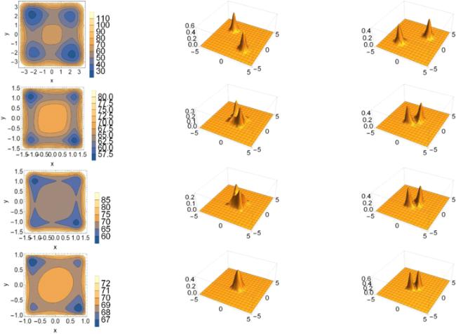
Figure 6. The contour plots of the potentials ${\Upsilon }^{(k)}\left(x,y\right)$ (left panel), the ground state probability density of the second configuration (medial panel), and the ground state probability density of the first configuration (right panel), as $k=0.05,$ $2.2,$ $3,$ and $10$ from top to bottom, obtained numerically. |
For asymmetric potential, the energy levels do not occur in quartets, and, except in a case of accidental degeneracy, the energies in one potential are different from those in the other. We have two configurations in the same system. The eigenfunctions near the bottom are localized in their respective wells (except when the barrier is low), but the wavefunctions close to the top of the barrier may extend through the classically forbidden region into the other wells. Conversely, for each symmetric two-dimensional double-minimum potential, the energy levels of both wells occur in pairs and have the same values. The eigenfunctions are delocalized, extending over both wells.
When two (or more) types of spectra associated with different configurations coexist in the same energy region, we call them coexistence phenomena. This circumstance occurs when configuration mixing due to tunneling is weak and the wave functions retain their localizations about different minima. In contrast, when the configuration mixing is strong, a large-amplitude configuration fluctuations (delocalization of the wave functions) extending to different local minima may occur.
For the ground state of the first and second configurations of the potential $\Upsilon ,$ the evolution of the probability density as a function of the variables $x$ and $y$ and the parameter $k$ is represented in figure 6. At $k=0.05,$ the probability density of the first configuration is composed of two separate peaks. By increasing the value of $k,$ the two peaks of the probability density become closely spaced. At $k\in [2.2,2.4],$ the probability density is composed of two pieces. When the state is in nearness to the top of the barrier, the tunneling is strong and the fluctuations phenomena take place, each piece of probability density becomes more extended over two minima and has a peak around the one minimum, however, its tail spreads to the other one. When the state is above the barrier, one obtains normal two peaks probability density with equal height, as presented in figure 6 (right panel).
Beginning from $k=0.05,$ the ground state probability density of the second configuration is composed of two separate peaks. With a decrease in the barrier height, the two separate peaks of the probability density become closely spaced. At a certain point, the ground state probability density forms an isolated island with the four unequal peaks that happens as a consequence of the strong tunneling between the potential wells. In this case, one says that two configurations coexist in the same system as well as in the same state. When the ground state of the second configuration is above the barrier, we have a single-peak probability density, as represented in figure 6 (medial panel). Depending on what was previously mentioned, with changing of $k,$ a transition is covered from coexistence phenomena of the two distinct TSMs to fluctuations phenomena with unequal peaks ending with the spectra of ${H}_{\alpha }.$
3. Non-CQOM
The nucleus is a quantum many-body system so that its shape is depending on the number of nucleons that exist in the nucleus and the nature of the interactions between the nucleons. For example, doubly magic nuclei, in their ground state, have a spherical shape. If this nuclear system is excited, or if more nucleons are added or subtracted, the spherical symmetry is distorted and the nucleus turns into a deformed shape (prolate or oblate). A major part of deformed nuclei exhibit quadrupole reflection-symmetric shapes, and their spectra are characterized by positive-parity bands. While, octupole reflection-asymmetric shapes (pear-like nuclei) exist in certain regions [14–20], either in an octupole deformation or octupole vibrations. Around neutron (proton) numbers, namely $N(Z)=34,56,88,$ and $134,$ the tendency towards octupolarity becomes stronger. The Rn isotopes, with A = 218–222, are the best examples of the octupole vibrators. However, the 222,224,226,228Ra and 224,226,228,230Th isotopes are typical octupole deformation.
Most studies of first- and second-order QSPT have paid more attention to quadrupole degrees of freedom, either for axially-symmetric deformed shapes or triaxial shapes. Much less analysis are the QSPTs connected to reflection-asymmetric shapes. Geometric collective models [28–31], algebraic models [32], and microscopic energy density functionals [33–36] have been used in studies of this type of QSPT. In [37, 38], the QSPT from octupole vibrations into octupole deformation has been considered. Additionally, the double QSPT was reported [39], between non-octupole and octupole-deformed shapes and simultaneously between spherical and quadrupole-deformed prolate shapes. A different critical point including quadrupole and octupole deformations have been suggested [28–31] expanding the idea of critical point introduced for studying positive parity states.
In the CQOM, the even–even nucleus can able to oscillate with respect to the quadrupole ${\beta }_{2}$ and octupole ${\beta }_{3}$ variables. The Hamiltonian of the CQOM can be written as8 ) does not contain the $\gamma $ degree of freedom. The potential function ${\rm{\Lambda }}$ consists of two parts. The first part, ${C}_{21}{\beta }_{2}^{2}/2+{C}_{31}{\beta }_{3}^{2}/2,$ generates HOP however the second part, $X(I)/({d}_{2}{\beta }_{2}^{2}+{d}_{3}{\beta }_{3}^{2}),$ produces an angular momentum dependent core. If (${\beta }_{2,\min },{\beta }_{3,\min }$) denotes the position of the bottom of the potential (8 ) such that ${\beta }_{2,\min }\ne 0$ and ${\beta }_{2,\min }\ne 0,$ the model parameters satisfy the following relation, ${d}_{2}/{C}_{21}={d}_{3}/{C}_{31}.$ In this situation, the shape of the bottom of the potential is an ellipse. If we consider the prolate quadrupole deformation ${\beta }_{2}\gt 0,$ the system oscillate between ${\beta }_{3}\gt 0$ and ${\beta }_{3}\lt 0$ along the ellipse surrounding the infinite potential core. It should be noted that, in the coherent approach, the model is limited to a specific category of exact analytic solutions. On the contrary, in the non-coherent case, the parameters are all allowed to vary without any constraint.
$\begin{eqnarray}H=-\displaystyle \frac{{\hslash }^{2}}{2{B}_{2}}\displaystyle \frac{{\partial }^{2}}{\partial {\beta }_{2}^{2}}-\displaystyle \frac{{\hslash }^{2}}{2{B}_{3}}\displaystyle \frac{{\partial }^{2}}{\partial {\beta }_{3}^{2}}+{\rm{\Lambda }}\left({\beta }_{2},{\beta }_{3},I\right),\end{eqnarray}$
Where $\begin{eqnarray}{\rm{\Lambda }}\left({\beta }_{2},{\beta }_{3},I\right)=\displaystyle \frac{1}{2}{C}_{21}{\beta }_{2}^{2}+\displaystyle \frac{1}{2}{C}_{31}{\beta }_{3}^{2}+\displaystyle \frac{X(I)}{{d}_{2}{\beta }_{2}^{2}+{d}_{3}{\beta }_{3}^{2}},\end{eqnarray}$
with $X(I)=[{d}_{0}+I(I+1)]/2.$ Here ${B}_{2}$ (${B}_{3}$), ${C}_{21}$ (${C}_{31}$) and ${d}_{2}$ (${d}_{3}$) are quadrupole (octupole) mass, stiffness, and inertia parameters, respectively, while ${d}_{0}$ determines the potential core at $I=0.$ The two-dimensional potential (From the results of section 2 , we realized that the potentials (4 ) and (5 ) are constructing bridges between the HOP and the purely AOPs, ${H}_{\alpha }.$ Furthermore, by changing the barrier height, we can have examples of the occurrence of fluctuations phenomena in the ground state and excited states. These essential ideas must be applied to the CQOM. It is fundamental to know how stable octupole deformation is, i.e. we need to know the size of fluctuations around the equilibrium value of ${\beta }_{3}.$ Moreover, in [40–42], the analysis of the octupole correlations was based on a simple one-dimensional model of octupole collective motion. The potential of this model has two minima, symmetric around ${\beta }_{3}=0$ and frozen quadrupole variable was considered. Depending on the height of the inner barrier between a reflection asymmetric shape and its mirror image a parity splitting arises. In such a way the explicit form of the potential in terms of the quadrupole ${\beta }_{2}$ and octupole ${\beta }_{3}$ deformation variables was not given. As a consequence, some basic characteristics of the quadrupole and octupole modes and their interaction remain outside of consideration such as the behavior of the system in dependence on the quadrupole and octupole stiffness. On the other hand, in CQOM [26, 27], the potential of the system depends on the two deformation variables ${\beta }_{2}$ and ${\beta }_{3}.$ The system is considered to oscillate between positive and negative ${\beta }_{3}$ values by rounding an infinite potential core in the (${\beta }_{2},$ ${\beta }_{3}$) plane with ${\beta }_{2}\gt 0.$ In this case, there is no barrier that seprates ${\beta }_{3}\gt 0$ and ${\beta }_{3}\lt 0$ after the quadrupole coordinate ${\beta }_{2}$ is let to vary. Hence, there is a need to suggest new potentials that have the advantages of the HOP and that generate a barrier separates ${\beta }_{3}\gt 0$ and ${\beta }_{3}\lt 0$ along the ${\beta }_{2}$ axis. The strength of barrier penetration controls the amount of shift in the energy of a negative-parity state with respect to the positive-parity one.
Here, we focus on the fluctuations phenomena through the barrier at ${\beta }_{3}=0$ in the space (${\beta }_{2},{\beta }_{3}$) and examine the evolution of the potential in dependence on both quadrupole and octupole degrees of freedom as well as on the collective angular momentum. To this end, we introduce the following effective potentials, using DLPs (4 ) and (5 ) in the quadrupole ${\beta }_{2}$ and octupole ${\beta }_{3}$ axial deformation variables
$\begin{eqnarray}\begin{array}{l}W\left({\beta }_{2},{\beta }_{3},I\right)=\displaystyle \frac{1}{2}{C}_{21}{\beta }_{2}^{4}+\displaystyle \frac{1}{2}{C}_{31}{\beta }_{3}^{4}+\displaystyle \frac{{C}_{22}}{{\beta }_{2}^{4}+{C}_{23}}\\ \,\,\,\,\,\,\,+\,\displaystyle \frac{{C}_{32}}{{\beta }_{3}^{4}+{C}_{33}}+\displaystyle \frac{X(I)}{{d}_{2}{\beta }_{2}^{2}+{d}_{3}{\beta }_{3}^{2}},\end{array}\end{eqnarray}$
$\begin{eqnarray}\begin{array}{l}Q\left({\beta }_{2},{\beta }_{3},I\right)=\displaystyle \frac{1}{2}{C}_{21}{\beta }_{2}^{2}+\displaystyle \frac{1}{2}{C}_{31}{\beta }_{3}^{2}+\displaystyle \frac{{C}_{22}}{{\beta }_{2}^{4}+{C}_{23}}\\ \,\,\,\,\,\,+\,\displaystyle \frac{{C}_{32}}{{\beta }_{3}^{4}+{C}_{33}}+\displaystyle \frac{X(I)}{{d}_{2}{\beta }_{2}^{2}+{d}_{3}{\beta }_{3}^{2}}.\end{array}\end{eqnarray}$
The shape of $W\left({\beta }_{2},{\beta }_{3},I\right)$ is illustrated in figure 7(a). It is characterized by two energy minima for ${\beta }_{3}\lt 0$ and ${\beta }_{3}\gt 0$ separated by a barrier. With increasing angular momentum, centrifugal forces modify the effective potential. This potential, thus, depends on the angular momentum. At ${\beta }_{3}=0,$ the height of the barrier, between ${\beta }_{3}\lt 0$ and ${\beta }_{3}\gt 0,$ depends on ${\beta }_{2}.$ The evolution of the vertical cross-sections of the potential (9a ) as a function of the angular momentum and ${\beta }_{2}$ variable is shown in figure 7(b), at ${\beta }_{3}=0.$
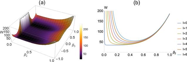
Figure 7. (a) The three-dimensional plot of the potential $W\left({\beta }_{2},{\beta }_{3},0\right).$ (b) The evolution of the vertical cross-sections of the potentials $W\left({\beta }_{2},{\beta }_{3},I\right),$ at ${\beta }_{3}=0,$ as a function of the angular momentum $I$ and ${\beta }_{2}.$ |
The model formalism with potentials (8 ) and (9 ) was applied to several nuclei, namely, 100Mo, 146,148Nd, 148,150Sm,220Ra, 220,222Rn, and 220,222Th. All selected nuclei are characterized by the energy ratio ${R}_{{4}_{1}^{+}/{2}_{1}^{+}}={E}_{{4}_{1}^{+}}/{E}_{{2}_{1}^{+}}$ in the range 2–2.5, the energy ratio ${R}_{{3}_{1}^{-}/{2}_{1}^{+}}={E}_{{3}_{1}^{-}}/{E}_{{2}_{1}^{+}}$ in the range 2–3.5, and the energy bands with alternating parity. From tables 1–5, good agreement has been found between the calculated and measured spectra.
Table 1. Theoretical and experimental energy spectra of 100Mo [43] and 146Nd [44], normalized to the energy of the first excited 2+ state. For each nucleus, the theoretical spectra ${{\epsilon }}_{i}^{Q},$ ${{\epsilon }}_{i}^{W},$ and ${{\epsilon }}_{i}^{{\rm{\Lambda }}}$ are the results from the potentials ( |
| 100Mo | 146Nd | ||||||||
|---|---|---|---|---|---|---|---|---|---|
| ${L}^{+}$ | ${{\epsilon }}_{i}^{\exp }$ | ${{\epsilon }}_{i}^{Q}$ | ${{\epsilon }}_{i}^{W}$ | ${{\epsilon }}_{i}^{{\rm{\Lambda }}}$ | ${{\epsilon }}_{i}^{\exp }$ | ${{\epsilon }}_{i}^{Q}$ | ${{\epsilon }}_{i}^{W}$ | ${{\epsilon }}_{i}^{{\rm{\Lambda }}}$ | |
| Yrast | ${0}^{+}$ | 0 | 0 | 0 | 0 | 0 | 0 | 0 | 0 |
| ${2}^{+}$ | 1 | 1 | 1 | 1 | 1 | 1 | 1 | 1 | |
| ${4}^{+}$ | 2.121 27 | 2.262 17 | 2.211 52 | 2.322 41 | 2.298 81 | 2.440 77 | 2.246 87 | 2.416 71 | |
| ${6}^{+}$ | 3.448 66 | 3.569 56 | 3.572 88 | 3.707 91 | 3.922 43 | 3.991 42 | 3.642 52 | 3.931 76 | |
| ${8}^{+}$ | 4.905 15 | 4.889 92 | 5.056 45 | 5.112 75 | 5.715 07 | 5.579 33 | 5.158 55 | 5.479 37 | |
| ${10}^{+}$ | (6.285 85) | (6.216 31) | (6.644 81) | (6.526 41) | 7.315 34 | 7.183 33 | 6.777 89 | 7.041 51 | |
| ${12}^{+}$ | (7.584 39) | (7.545 76) | (8.325 69) | (7.944 75) | 8.800 57 | 8.796 12 | 8.488 65 | 8.611 64 | |
| ${14}^{+}$ | (9.101 38) | (8.876 95) | (10.0899) | (9.365 87) | 10.3442 | 10.4142 | 10.2820 | 10.1867 | |
| ${16}^{+}$ | 12.0328 | 12.0355 | 12.1508 | 11.7653 | |||||
| Yrast | ${1}^{-}$ | ||||||||
| ${3}^{-}$ | 3.562 92 | 1.6204 | 1.584 62 | 1.647 13 | 2.621 42 | 1.697 97 | 1.602 24 | 1.687 77 | |
| ${5}^{-}$ | (4.368 55) | (2.913 45) | (2.875 53) | (3.011 49) | 3.3442 | 3.208 84 | 2.928 27 | 3.167 98 | |
| ${7}^{-}$ | (5.308 44) | (4.228 70) | (4.300 64) | (4.408 82) | 4.472 01 | 4.782 61 | 4.386 72 | 4.703 08 | |
| ${9}^{-}$ | (6.159 82) | (5.552 60) | (5.838 39) | (5.818 81) | 5.963 42 | 6.379 91 | 5.956 14 | 6.259 15 | |
| ${11}^{-}$ | (7.529 31) | (6.880 75) | (7.474 31) | (7.235 14) | 7.714 19 | 7.988 90 | 7.622 45 | 7.825 82 | |
| ${13}^{-}$ | (9.222 93) | (8.211 19) | (9.197 88) | (8.655 04) | 9.464 52 | 9.604 62 | 9.375 46 | 9.398 68 | |
| ${15}^{-}$ | 11.1457 | 11.2245 | 11.2073 | 10.9756 | |||||
| Non-yrast | ${2}^{+}$ | 1.297 80 | 1.183 20 | 0.680 92 | 2.212 67 | 2.017 19 | 1.445 47 | 0.686 05 | 2.458 43 |
| ${4}^{+}$ | 2.733 20 | 1.609 49 | 1.146 30 | 2.625 27 | 2.871 75 | 2.444 63 | 1.686 05 | 3.457 11 | |
| ${6}^{+}$ | (3.307 32) | (2.182 94) | (1.680 92) | (3.211 91) | 3.845 75 | 3.886 04 | 2.932 92 | 4.874 89 | |
| $2{B}_{2}/{\hslash }^{2}$ | 2.000 00 | 12.0000 | 1.500 00 | 0.900 00 | 7.000 00 | 1.000 00 | |||
| Δ | 0.779 32 | 0.835 37 | 0.708 31 | 0.463 95 | 0.628 83 | 0.542 15 | |||
| 148Nd | 148Sm | ||||||||
|---|---|---|---|---|---|---|---|---|---|
| L+ | ${{\epsilon }}_{i}^{\exp }$ | ${{\epsilon }}_{i}^{Q}$ | ${{\epsilon }}_{i}^{W}$ | ${{\epsilon }}_{i}^{{\rm{\Lambda }}}$ | ${{\epsilon }}_{i}^{\exp }$ | ${{\epsilon }}_{i}^{Q}$ | ${{\epsilon }}_{i}^{W}$ | ${{\epsilon }}_{i}^{{\rm{\Lambda }}}$ | |
| Yrast | ${0}^{+}$ | 0 | 0 | 0 | 0 | 0 | 0 | 0 | 0 |
| ${2}^{+}$ | 1 | 1 | 1 | 1 | 1 | 1 | 1 | 1 | |
| ${4}^{+}$ | 2.493 54 | 2.553 08 | 2.502 60 | 2.416 71 | 2.144 83 | 2.236 68 | 2.1853 | 2.238 27 | |
| ${6}^{+}$ | 4.241 96 | 4.268 11 | 4.213 86 | 3.931 76 | 3.463 38 | 3.511 07 | 3.526 06 | 3.513 97 | |
| ${8}^{+}$ | 6.152 47 | 6.045 56 | 6.064 29 | 5.479 37 | 4.933 67 | 4.796 40 | 4.993 45 | 4.801 10 | |
| ${10}^{+}$ | (8.190 92) | (7.850 48) | (8.027 51) | (7.041 51) | 6.175 00 | 6.086 76 | 6.568 94 | 6.093 38 | |
| ${12}^{+}$ | (10.2957) | (9.670 09) | (10.0889) | (8.611 64) | 7.458 48 | 7.379 64 | 8.239 52 | 7.388 34 | |
| ${14}^{+}$ | 8.731 96 | 8.673 94 | 9.995 50 | 8.684 87 | |||||
| ${16}^{+}$ | 9.988 01 | 9.969 14 | 11.8294 | 9.982 40 | |||||
| Yrast | ${1}^{-}$ | 3.391 45 | 0.378 19 | 0.391 79 | 0.397 02 | ||||
| ${3}^{-}$ | 3.312 33 | 1.744 68 | 1.717 02 | 1.687 77 | 2.110 67 | 1.609 20 | 1.570 78 | 1.610 30 | |
| ${5}^{-}$ | 4.117 67 | 3.398 94 | 3.338 22 | 3.167 98 | 2.896 97 | 2.871 87 | 2.838 37 | 2.874 01 | |
| ${7}^{-}$ | 5.450 78 | 5.152 03 | 5.123 77 | 4.703 08 | 3.868 07 | 4.152 85 | 4.245 25 | 4.156 64 | |
| ${9}^{-}$ | 7.065 96 | 6.945 65 | 7.032 86 | 6.259 15 | 5.101 58 | 5.441 16 | 5.768 59 | 5.446 80 | |
| ${11}^{-}$ | (8.871 06) | (8.758 89) | (9.046 62) | (7.825 82) | 6.568 78 | 6.732 97 | 7.393 01 | 6.740 62 | |
| ${13}^{-}$ | (10.8300) | (10.5835) | (11.1532) | (9.398 68) | 7.991 64 | 8.026 65 | 9.107 35 | 8.036 45 | |
| ${15}^{-}$ | 9.333 27 | 9.321 45 | 10.9031 | 9.333 53 | |||||
| Non-yrast | ${2}^{+}$ | 3.039 11 | 1.640 91 | 0.785 20 | 2.458 43 | 2.588 59 | 1.149 78 | 0.684 21 | 2.014 85 |
| ${4}^{+}$ | 3.881 34 | 2.639 76 | 1.785 16 | 3.457 11 | 3.015 45 | 2.149 59 | 1.684 21 | 3.014 55 | |
| ${6}^{+}$ | 5.316 87 | 4.193 52 | 3.287 79 | 4.874 89 | 3.443 21 | 3.386 47 | 2.869 51 | 4.253 16 | |
| $2{B}_{2}/{\hslash }^{2}$ | 0.6000 | 1.200 00 | 1.000 00 | 2.300 00 | 26.0000 | 2.300 00 | |||
| Δ | 0.829 121 | 0.905 12 | 0.966 31 | 0.485 58 | 0.862 96 | 0.424 24 | |||
| 150Sm | 220Ra | ||||||||
|---|---|---|---|---|---|---|---|---|---|
| ${L}^{+}$ | ${{\epsilon }}_{i}^{\exp }$ | ${{\epsilon }}_{i}^{Q}$ | ${{\epsilon }}_{i}^{W}$ | ${{\epsilon }}_{i}^{{\rm{\Lambda }}}$ | ${{\epsilon }}_{i}^{\exp }$ | ${{\epsilon }}_{i}^{Q}$ | ${{\epsilon }}_{i}^{W}$ | ${{\epsilon }}_{i}^{{\rm{\Lambda }}}$ | |
| Yrast | ${0}^{+}$ | 0 | 0 | 0 | 0 | 0 | 0 | 0 | 0 |
| ${2}^{+}$ | 1 | 1 | 1 | 1 | 1 | 1 | 1 | 1 | |
| ${4}^{+}$ | 2.315 57 | 2.472 05 | 2.361 23 | 2.416 71 | 2.297 48 | 2.553 08 | 2.432 83 | 2.393 24 | |
| ${6}^{+}$ | 3.829 04 | 4.067 41 | 3.886 13 | 3.931 76 | 3.854 90 | 4.268 11 | 4.049 04 | 3.875 43 | |
| ${8}^{+}$ | 5.500 00 | 5.706 27 | 5.534 38 | 5.479 37 | 5.608 96 | 6.045 56 | 5.794 85 | 5.386 40 | |
| ${10}^{+}$ | 7.285 03 | 7.363 85 | 7.287 12 | 7.041 51 | 7.522 13 | 7.850 48 | 7.648 49 | 6.910 28 | |
| ${12}^{+}$ | 9.126 95 | 9.031 62 | 9.132 18 | 8.611 64 | 9.586 55 | 9.670 09 | 9.596 82 | 8.441 20 | |
| ${14}^{+}$ | 11.0057 | 10.7055 | 11.0607 | 10.1867 | 11.7966 | 11.4987 | 11.6306 | 9.976 41 | |
| ${16}^{+}$ | 13.1326 | 12.3834 | 13.0658 | 11.7653 | 14.1373 | 13.3332 | 13.7428 | 11.5146 | |
| ${18}^{+}$ | 16.5933 | 15.1718 | 15.9278 | 13.0552 | |||||
| Yrast | ${1}^{-}$ | (2.313 73) | (0.378 20) | (0.404 39) | (0.400 87) | ||||
| ${3}^{-}$ | 3.207 78 | 1.711 20 | 1.655 40 | 1.687 77 | (2.656 58) | (1.744 68) | (1.686 97) | (1.677 74) | |
| ${5}^{-}$ | 4.064 97 | 3.261 34 | 3.106 63 | 3.167 98 | (3.556 30) | (3.398 94) | (3.222 72) | (3.128 80) | |
| ${7}^{-}$ | 5.284 13 | 4.883 60 | 4.696 23 | 4.703 08 | (4.890 76) | (5.152 03) | (4.907 40) | (4.628 72) | |
| ${9}^{-}$ | 6.683 83 | 6.533 41 | 6.398 55 | 6.259 15 | (6.519 89) | (6.945 65) | (6.709 13) | (6.147 20) | |
| ${11}^{-}$ | 8.216 77 | 8.196 77 | 8.198 72 | 7.825 82 | (8.381 51) | (8.758 89) | (8.611 46) | (7.675 08) | |
| ${13}^{-}$ | 9.860 18 | 9.867 98 | 10.0865 | 9.398 68 | (10.4409) | (10.5835) | (10.6035) | (9.208 37) | |
| ${15}^{-}$ | 11.7189 | 11.5441 | 12.0541 | 10.9756 | (12.6751) | (12.4153) | (12.6773) | (10.7452) | |
| ${17}^{-}$ | (15.0706) | (14.2520) | (14.8265) | (12.2846) | |||||
| Non-yrast | ${2}^{+}$ | 2.217 07 | 2.496 15 | 1.721 49 | 3.457 11 | ||||
| ${4}^{+}$ | 3.132 04 | 3.968 87 | 3.082 73 | 4.874 89 | |||||
| $2{B}_{2}/{\hslash }^{2}$ | 0.800 00 | 2.600 00 | 1.000 00 | 0.600 00 | 1.700 00 | 1.100 00 | |||
| Δ | 0.593 81 | 0.529 96 | 0.810 63 | 0.719 99 | 0.574 23 | 1.072 01 | |||
| 220Rn | 220Th | ||||||||
|---|---|---|---|---|---|---|---|---|---|
| ${L}^{+}$ | ${{\epsilon }}_{i}^{\exp }$ | ${{\epsilon }}_{i}^{Q}$ | ${{\epsilon }}_{i}^{W}$ | ${{\epsilon }}_{i}^{{\rm{\Lambda }}}$ | ${{\epsilon }}_{i}^{\exp }$ | ${{\epsilon }}_{i}^{Q}$ | ${{\epsilon }}_{i}^{W}$ | ${{\epsilon }}_{i}^{{\rm{\Lambda }}}$ | |
| Yrast | ${0}^{+}$ | 0 | 0 | 0 | 0 | 0 | 0 | 0 | 0 |
| ${2}^{+}$ | 1 | 1 | 1 | 1 | 1 | 1 | 1 | 1 | |
| ${4}^{+}$ | 2.214 52 | 2.413 83 | 2.201 39 | 2.416 71 | 2.652 01 | 2.390 34 | 2.204 27 | 2.372 51 | |
| ${6}^{+}$ | (3.626 14) | (3.926 53) | (3.553 91) | (3.931 76) | 4.069 81 | 3.870 33 | 3.559 24 | 3.826 03 | |
| ${8}^{+}$ | (5.163 07) | (5.471 61) | (5.029 76) | (5.479 37) | 5.578 36 | 5.378 80 | 5.037 17 | 5.305 25 | |
| ${10}^{+}$ | (6.768 05) | (7.030 76) | (6.611 25) | (7.041 51) | 7.025 13 | 6.899 77 | 6.620 47 | 6.796 08 | |
| ${12}^{+}$ | (8.439 42) | (8.597 60) | (8.285 93) | (8.611 64) | 8.523 21 | 8.427 56 | 8.296 74 | 8.293 19 | |
| ${14}^{+}$ | (10.1772) | (10.1690) | (10.0445) | (10.1867) | 10.0698 | 9.959 36 | 10.0567 | 9.794 08 | |
| ${16}^{+}$ | (11.9793) | (11.7433) | (11.8796) | (11.7653) | 11.7850 | 11.4937 | 11.8931 | 11.2975 | |
| ${18}^{+}$ | (13.7979) | (13.3196) | (13.7854) | (13.3468) | 13.4977 | 13.0297 | 13.8001 | 12.8031 | |
| ${20}^{+}$ | (15.6178) | (14.8973) | (15.7571) | (14.9314) | 15.0771 | 14.5670 | 15.7729 | 14.3106 | |
| Yrast | ${1}^{-}$ | 2.669 71 | 0.397 09 | 0.470 03 | 0.397 02 | ||||
| ${3}^{-}$ | 2.751 04 | 1.686 46 | 1.579 42 | 1.687 77 | |||||
| ${5}^{-}$ | (3.534 85) | (3.163 84) | (2.860 83) | (3.167 98) | 3.468 76 | 3.124 75 | 2.864 98 | 3.094 33 | |
| ${7}^{-}$ | (4.681 33) | (4.696 66) | (4.277 69) | (4.703 08) | 4.638 74 | 4.622 44 | 4.284 09 | 4.563 66 | |
| ${9}^{-}$ | (6.066 80) | (6.249 93) | (5.808 17) | (6.259 15) | 5.999 65 | 6.138 18 | 5.816 51 | 6.049 64 | |
| ${11}^{-}$ | (7.609 96) | (7.813 46) | (7.437 58) | (7.825 82) | 7.535 43 | 7.663 04 | 7.447 62 | 7.544 05 | |
| ${13}^{-}$ | (9.241 08) | (9.382 87) | (9.155 21) | (9.398 68) | 8.918 67 | 9.193 08 | 9.166 75 | 9.043 25 | |
| ${15}^{-}$ | (10.9473) | (10.9559) | (10.9529) | (10.9756) | 10.4880 | 10.7263 | 10.9658 | 10.5455 | |
| ${17}^{-}$ | (12.7328) | (12.5312) | (12.8240) | (12.5557) | 12.1019 | 12.2615 | 12.8381 | 12.0501 | |
| ${19}^{-}$ | (14.5635) | (14.1083) | (14.7633) | (14.1387) | 13.8000 | 13.7983 | 14.7785 | 13.5566 | |
| ${21}^{-}$ | (16.4378) | (15.6865) | (16.7663) | (15.7250) | |||||
| $2{B}_{2}/{\hslash }^{2}$ | 1.000 00 | 15.0000 | 1.000 00 | 1.100 00 | 14.0000 | 1.200 00 | |||
| Δ | 0.630 22 | 0.556 52 | 0.627 32 | 0.444 85 | 0.620 04 | 0.498 08 | |||
| 222Rn | 222Th | ||||||||
|---|---|---|---|---|---|---|---|---|---|
| ${L}^{+}$ | ${{\epsilon }}_{i}^{\exp }$ | ${{\epsilon }}_{i}^{Q}$ | ${{\epsilon }}_{i}^{W}$ | ${{\epsilon }}_{i}^{{\rm{\Lambda }}}$ | ${{\epsilon }}_{i}^{\exp }$ | ${{\epsilon }}_{i}^{Q}$ | ${{\epsilon }}_{i}^{W}$ | ${{\epsilon }}_{i}^{{\rm{\Lambda }}}$ | |
| Yrast | ${0}^{+}$ | 0 | 0 | 0 | 0 | 0 | 0 | 0 | 0 |
| ${2}^{+}$ | 1 | 1 | 1 | 1 | 1 | 1 | 1 | 1 | |
| ${4}^{+}$ | 2.408 16 | 2.632 37 | 2.508 07 | 2.393 24 | 2.399 35 | 2.613 24 | 2.485 67 | 2.393 24 | |
| ${6}^{+}$ | (4.127 28) | (4.471 30) | (4.227 00) | (3.875 43) | 4.091 65 | 4.421 55 | 4.173 37 | 3.875 43 | |
| ${8}^{+}$ | (6.058 54) | (6.395 41) | (6.086 01) | (5.386 40) | 5.965 63 | 6.309 13 | 5.997 56 | 5.386 40 | |
| ${10}^{+}$ | (8.125 67) | (8.358 83) | (8.058 28) | (6.910 28) | 7.971 09 | 8.232 81 | 7.933 18 | 6.910 28 | |
| ${12}^{+}$ | (10.2760) | (10.3431) | (10.1290) | (8.441 20) | 10.0966 | 10.1757 | 9.966 02 | 8.441 20 | |
| ${14}^{+}$ | (12.4447) | (12.3403) | (12.2884) | (9.976 41) | 12.3279 | 12.1303 | 12.0864 | 9.976 41 | |
| ${16}^{+}$ | (14.6493) | (14.3460) | (14.5288) | (11.5146) | 14.6634 | 14.0928 | 14.2870 | 11.5146 | |
| ${18}^{+}$ | 17.0949 | 16.0609 | 16.5621 | 13.0552 | |||||
| Yrast | ${1}^{-}$ | 3.226 10 | 0.369 99 | 0.390 91 | 0.400 87 | ||||
| ${3}^{-}$ | 3.411 92 | 1.776 19 | 1.719 35 | 1.677 74 | 2.547 74 | 1.768 71 | 1.709 79 | 1.677 74 | |
| ${5}^{-}$ | (4.284 64) | (3.536 43) | (3.347 36) | (3.128 80) | 3.551 55 | 3.502 96 | 3.310 01 | 3.128 80 | |
| ${7}^{-}$ | (5.634 80) | (5.426 52) | (5.141 12) | (4.628 72) | 5.038 19 | 5.359 05 | 5.070 37 | 4.628 72 | |
| ${9}^{-}$ | (7.287 33) | (7.373 73) | (7.059 07) | (6.147 20) | 6.848 34 | 7.267 86 | 6.952 47 | 6.147 20 | |
| ${11}^{-}$ | (9.174 01) | (9.349 01) | (9.082 05) | (7.675 08) | 8.852 15 | 9.202 43 | 8.938 13 | 7.675 08 | |
| ${13}^{-}$ | (11.2197) | (11.3404) | (11.1981) | (9.208 37) | 10.9956 | 11.1518 | 11.0157 | 9.208 37 | |
| ${15}^{-}$ | (13.3475) | (13.3422) | (13.3988) | (10.7452) | 13.2646 | 13.1107 | 13.1770 | 10.7452 | |
| ${17}^{-}$ | (15.4774) | (15.3513) | (15.6777) | (12.2846) | 15.6738 | 15.0763 | 15.4155 | 12.2846 | |
| ${19}^{-}$ | (17.6472) | (17.3659) | (18.0295) | (13.8264) | |||||
| ${21}^{-}$ | (19.8502) | (19.3850) | (20.4501) | (15.3708) | |||||
| $2{B}_{2}/{\hslash }^{2}$ | 0.460 00 | 1.170 00 | 1.100 00 | 0.490 00 | 1.300 00 | 1.100 00 | |||
| Δ | 0.661 79 | 0.659 05 | 1.358 38 | 0.586 92 | 0.432 97 | 1.196 41 | |||
The energy levels are determined by (7 ) and potentials (8 ) and (9 ). The two-dimensional Schrödinger equation is solved for each value of $I=0,1,2,\ldots $ separately. The energy spectrum is normalized to ${2}_{1}^{+}$ state of the ground state band such that
$\begin{eqnarray}{{\epsilon }}_{{I}^{\pm }}^{{\rm{th}}}=\displaystyle \frac{{E}_{{I}^{\pm }}^{{\rm{th}}}-{E}_{{0}^{+}}^{{\rm{th}}}}{{E}_{{2}^{+}}^{{\rm{th}}}-{E}_{{0}^{+}}^{{\rm{th}}}}.\end{eqnarray}$
The root mean absolute error is defined as, ${\rm{\Delta }}=\sqrt{\displaystyle \sum _{i}\left|{{\epsilon }}_{i}^{\exp }-{{\epsilon }}_{i}^{{\rm{th}}}\right|/{n}_{l}},$ where ${E}_{i}^{\exp }$ and ${E}_{i}^{{\rm{th}}}$ are the experimental and calculated energies of the ith level and ${n}_{l}$ represents the number of levels. Δ is one of the important statistical quantities which is used for the validation of the predicted result. Once the diagonalizations, using the finite-difference method, have been accomplished for all angular momenta, one gets a spectrum and can determine the value of Δ. Then the parameters ${C}_{2i},$ ${C}_{3i},$ ${d}_{2},$ ${d}_{3},$ ${d}_{0},$ $i=1,2,3$ and the boundaries parameters ${\beta }_{2b}$ and ${\beta }_{3b}$ of the finite-difference method can be adjusted to give the best description of experimental energies.
By following this procedure, we can have the best fitting of experimental data of an individual nucleus. However, we choose to go a step further and search for the global parametrization (maximum common parameters of a set of nuclei with a minimum value of Δ). As an alternative approach, we searched for a simplified global CQOM parametrization for selected octupole nuclei that belong to different regions in the nuclear landscape. This set of global parameters leads to a description of about 200 collective levels in 10 nuclei with a root mean absolute error from the observed level energies less than 0.7. In this approach, all the model parameters are constants except ${B}_{2}.$ For the best fitting of experimental data, the value of ${B}_{2}$ must be adjusted. The values of the global CQOM parameters of the potentials (8 ) and (9 ) are tabulated in table 6. The idea of global parametrization is not new. This technique was applied to many isotope series in the study of exotic nuclei [45].
Table 6. The parameters of the potentials ${\rm{\Lambda }}\left({\beta }_{2},{\beta }_{3},I\right),$ $W\left({\beta }_{2},{\beta }_{3},I\right)$ and $Q\left({\beta }_{2},{\beta }_{3},I\right)$ are ${B}_{3},$ ${d}_{2},$ and ${d}_{3}$ (in ${\hslash }^{2}$ MeV−1), ${d}_{0}\,$(in ${\hslash }^{2}$), ${C}_{21}$ and ${C}_{31}$ (in MeV), ${C}_{22}={C}_{32}$ = 1 MeV, whereas ${C}_{23}$ and ${C}_{33}$ are dimensionless, ${C}_{23}=1.$ |
| $2{B}_{3}/{\hslash }^{2}$ | ${C}_{21}$ | ${C}_{31}$ | ${C}_{33}$ | ${d}_{2}$ | ${d}_{3}$ | ${d}_{0}$ | |
|---|---|---|---|---|---|---|---|
| ${\rm{\Lambda }}\left({\beta }_{2},{\beta }_{3},I\right)$ | 1 | 300 | 240 | — | 6 | 0.0005 | 0.1 |
| $W\left({\beta }_{2},{\beta }_{3},I\right)$ | 1 | 300 | 200 | 0.03 | 7 | 0.000 02 | 0.01 |
| $Q\left({\beta }_{2},{\beta }_{3},I\right)$ | 0.4 | 300 | 240 | 0.015 | 6 | 0.0002 | 0.1 |
At ${\beta }_{3}=0,$ for a small value of quadrupole ${\beta }_{2}$ variable, the height of the barrier is very high. With increasing ${\beta }_{2},$ the height decreases. At some point, it reaches its minimum value. Increasing further the ${\beta }_{2}$ variable, the height of the barrier is increasing again. This geometric analysis suggests that the oscillations of the system in the two-dimensional case of simultaneous manifestations of the quadrupole and octupole modes are performed in a different way, compared to the one-dimensional case of a reflection asymmetric shape with a frozen quadrupole variable. The presence of a tunneling effect in the space of the octupole variable ${\beta }_{3}$ is sensitive to the quadrupole ${\beta }_{2}$ variable. Straightforwardly, in the (${\beta }_{2},{\beta }_{3}$) space, the strength of the tunneling through the barrier of each wave function varies with quadrupole ${\beta }_{2}$ variable. As a result, the parity shift effect observed in nuclear alternating parity bands, which can be explained as a result of the tunneling through the barrier, depends on the height of the barrier. Thus, not only the shape of wave function but also the energy spectrum are sensitive to the height of the barrier.
The comments on the model results are as follows:
The spectra of ten even–even nuclei characterized by yrast and non-yrast energy sequences with alternating parity and the energy ratio ${R}_{{4}_{1}^{+}/{2}_{1}^{+}}$ in the range 2–2.5 are discussed within the framework of CQOM. A satisfactory degree of agreement is obvious between the calculated energy spectra and the corresponding experimental values. In general, the results of HOP with barriers in its structure (9b ) suggest more exact outcomes, i.e. minimum Δ values, in comparison with the pure HOP predictions.
As seen in figure 8 and tables 1–5 the odd–even staggering is significant only for the lowest three odd levels, the positive-parity states (even levels) are extremely well reproduced, as well as the rest of the negative-parity states (odd ones). From figure 8, we can understand why global parametrization was able to generate the spectra of nuclei from different regions. These spectra are very close and look like lines with different slopes and starting from one point.
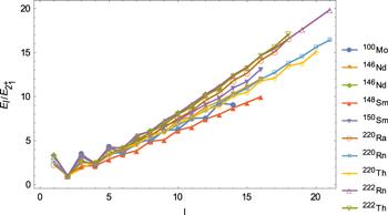
Figure 8. Experimental energy ratios ${E}_{{I}^{\pi }}/{E}_{{2}_{1}^{+}}$ for states of the positive-parity ground state band ($I$ even) and the lowest negative-parity band ($I$ odd), as functions of the angular momentum $I,$ for 100Mo [43], 146Nd [44], 148Nd [46], 148Sm [46], 150Sm [47], 220Ra [48], 220Rn [48], 220Th [48], 222Rn [49] and 222Th [49]. |
These results are in agreement with the findings of research [29]. In this work, an analytic, parameter-free solution of the Bohr Hamiltonian involving axially symmetric quadrupole and octupole deformations, as well as an infinite well potential, was obtained. This is done after separating variables in a way reminiscent of the variable moment of inertia concept. They find that the positive-parity states are extremely well-reproduced as well as the negative-parity states with the exception of the first three negative-parity levels. A similar phenomenon exists in the interacting boson model. In [50, 51], the level energy spectra of a set of 26 nuclei presenting a vibrational structure were analyzed using a simple U(5) prescription in the interacting boson model. It was observed that the ${2}_{1}^{+}$ energies are quite generally about 15% lower than expected from the global nuclear properties. The origin of this observed phenomenon is not clear. One hypothesis would be that some interactions not included in the standard interacting boson model have to be considered. In our case, a more complete investigation, including also more nuclei, should be performed to test the reality of such interaction which would be expected to depend on angular momenta and parity of the levels. It also decreases with the increase of the angular momenta of negative parity levels.
For most nuclei considered here, the yrast positive- and negative-parity states belong to a single band, that is, the two bands are located close in energy which is the hallmark of octupole deformation. In this case, the existence of the barrier between ${\beta }_{3}\lt 0$ and ${\beta }_{3}\gt 0$ is essential in the description of octupole deformation nuclei. This explains why the potential (9b ) suggests more exact outcomes.
The oscillations of the system in the two-dimensional case of the simultaneous manifestation of the quadrupole and octupole modes are performed in a different way, compared to the one-dimensional case of a reflection asymmetric shape with a frozen quadrupole variable. The height of the barrier of the potentials (9a ) and (9b) changes with quadrupole ${\beta }_{2}$ variable which controls the shape of the wave function. For the small value of quadrupole ${\beta }_{2}$ variable, the height of the barrier is very high, there is no tunneling through the barrier. With increasing ${\beta }_{2},$ the height decreases and one can have cases of the fluctuations phenomena in the wave function. The wave function extends over the two minima and has two peaks around the two minima, as well as the corresponding probability density. Increasing further the ${\beta }_{2}$ variable, the height of the barrier is increasing again.
In this case, there is no tunneling through the barrier. Figure 9 represents the ground state wave function of the nuclei considered in this work, using the potential (9b ). The peaks of the wave function begin to merge, however still distinguishable, for 100Mo, 146,148Nd, and 148,150Sm. For 220Ra, 220,222Rn, and 220,222Th, the ground state wave function posses a broader peak engulfing both wells of the associated effective potential.

Figure 9. The contour plots of the ground state wave functions of 100Mo, 146,148Nd, 148,150Sm, 220Ra, 220,222Rn, and 220,222Th using the potential ( |
The correspondence between the ground state bands of the current scheme, using (9a ), and X(5)-${\beta }^{4}$ model are indeed so close because the two models are derived from the collective Bohr–Mottelson Hamiltonian and employ quartic ${\beta }^{4}$ potential. Besides, the quadrupole degree of freedom, that associated with the two models, is expected to play an essential role in the description of the properties of the ground-state band. Obviously, the potential (9a ) can be viewed as an extension of X(5)-${\beta }^{4}$ model [6], where the octupole degree of freedom is considered for the sake of the negative parity bands, and at the same time the $\gamma $ degree of freedom is ignored to make the problem more tractable.
4. Conclusions
The nine-point finite difference method is used for the diagonalization of the Hamiltonian with DLPs. These potentials can evolve from wide spherical minima separated by high barriers to the near flat case or HOP. The spectra of DLPs (4 ) and (5) show a transition from TSM to the spectra of purely AOPs or HOP, and concurrently present many new features, such as the coexistence phenomena and fluctuations phenomena in the ground state and excited states. We had a ground state wave function with a four-peak structure. It is essential to distinguish between two types of potentials. For asymmetric potential, two or more configurations coexisted in the same system as well as in the same state and the fluctuations phenomena are characterized by the existence of peaks with unequal heights in the same wave function. In contrast, for symmetric potential, one configuration existed, the eigenfunctions were delocalized and the fluctuations phenomena were characterized by the existence of peaks with equal heights in the same wave function. Using these potentials, we shift the analysis of the coexistence phenomena and fluctuations phenomena from one that focuses on ISWP to one that focuses on HOP and purely AOPs.
Furthermore, by using DLPs in a CQOM Hamiltonian, we provide a global description of yrast and non-yrast bands with alternating parity in a set of even–even nuclei, namely, 100Mo, 146,148Nd, 148,150Sm, 220Ra, 220,222Rn, and 220,222Th. The global CQOM parametrization for selected octupole nuclei is achieved. We also obtained a ground state wave function with a two-peak structure. It is important to point out that, and this is the central focus of the present work, the existence of the barrier between ${\beta }_{3}\lt 0$ and ${\beta }_{3}\gt 0$ plays the central role in the study of the quadrupole–octupole deformed nuclei. The wave function shape is a reflection of the shape of the potential.