


1. Introduction
 -expansion approach [21, 22], the extended trial equation method (ETEM) [23], the improved tan (φ(ξ)/2)-expansion method (ITEM) [24], optimal homotopy and the differential transform method [25], the homogeneous balance method [26], the modified Kudryashov method [27], Riccati–Bernoulli sub-ODE method [28], the exp (− φ(ξ))-expansion method [29, 30], and the unified method and its generalized form [31–37].
 and n in the normal form, respectively. Here, we supervise the method of dynamical models concerning the ISW with the effect of the ponderomotive force owing to the high-frequency area, as well as for the LW, which is one variety of nonlinear wave models. The implementation of novel types of soliton solutions for the LW and ISWs has an extremely prominent status through the contributors. A few studies have converged on the Langmuir solitons. Musher et al [40] give support to the application of the weak turbulence hypothesis to LW turbulence, and consideration was given to plasma under relative unmagnetized and magnetized electron and ion temperatures. Zakharov [41] expressed the method of dynamical models for the LW. Benilov [42] illustrated the stability of solitons through the Zakharov model, that recognizes the interaction between ISWs and LWs. In [38, 40], a system of equations for the ISW under the action of the ponderomotive force due to the high-frequency field and the LW was discussed.
 -expansion method [22, 43]. The essential advantage of this technique over the other methods in the literature is that it provides novel explicit analytical wave solutions, including many real free parameters. The closed-form wave solutions of nonlinear NPDEs have their significant meaning to reveal the interior device of the physical phenomena. Furthermore, the calculations in this method are very simple and vital to providing new solutions compared to the steps in other approaches.
2. A brief description of the modified $\left(\tfrac{G^{\prime} }{G}\right)$  -expansion scheme

| • | Postulation 1: calculate m using the rule of the homogeneous analysis in ( |
| • | Postulation 2: the modified $\left(\tfrac{G^{\prime} }{G}\right)$ $\begin{eqnarray}h(\xi )=\displaystyle \sum _{i=-m}^{m}{A}_{i}{{\rm{\Theta }}}^{i},\end{eqnarray}$ where ${\rm{\Theta }}=\left(\tfrac{{G}^{{\prime} }}{G}+\tfrac{\lambda }{2}\right)$  , ∣A−m∣ + ∣Am∣ ≠ 0 and G = G(ξ) is given by , ∣A−m∣ + ∣Am∣ ≠ 0 and G = G(ξ) is given by $\begin{eqnarray}{G}^{{\prime\prime} }+\lambda {G}^{{\prime} }+\mu G=0,\end{eqnarray}$ where Ai, $\delta$ and $\mu$ are free parameters. From ( $\begin{eqnarray}{\rm{\Theta }}^{\prime} =b-{{\rm{\Theta }}}^{2},\end{eqnarray}$ where $b=\tfrac{{\lambda }^{2}-4\mu }{4}$  . So, Θ now satisfies the Riccati-like equation ( . So, Θ now satisfies the Riccati-like equation (If b > 0, then $\begin{eqnarray}{\rm{\Theta }}=\sqrt{b}\tanh (\sqrt{b}\xi ),\end{eqnarray}$ $\begin{eqnarray}{\rm{\Theta }}=\sqrt{b}\coth (\sqrt{b}\xi ),\end{eqnarray}$ If b = 0, then $\begin{eqnarray}{\rm{\Theta }}=\displaystyle \frac{1}{\xi },\end{eqnarray}$ If b < 0, then $\begin{eqnarray}{\rm{\Theta }}=-\sqrt{-b}\tan (\sqrt{-b}\xi ),\end{eqnarray}$ $\begin{eqnarray}{\rm{\Theta }}=\sqrt{-b}\cot (\sqrt{-b}\xi ).\end{eqnarray}$ |
| • | Postulation 3: inserting ( |

3. Soliton solutions for the model system related to ISWs and LWs
 and $U^{\prime\prime} =\tfrac{{{\rm{d}}}^{2}U}{{\rm{d}}{\xi }^{2}}$
  . Applying the homogeneous balance condition on
 | • | Result 1: $q=\pm \tfrac{\sqrt{4\mu {r}^{2}-2{p}^{2}-{\lambda }^{2}{r}^{2}}}{2}$ $\begin{eqnarray*}\begin{array}{rcl}{E}_{11}(x,t) & = & {{\rm{e}}}^{{\rm{i}}({px}+{qt})}\left[\displaystyle \frac{{f}_{1}r\sqrt{{\lambda }^{2}-4\mu }}{2}\right.\\ & & \times \ \left.\coth \left\{\displaystyle \frac{\sqrt{{\lambda }^{2}-4\mu }}{2}({rx}+{st})\right\}\right],\\ {n}_{11}(x,t) & = & \displaystyle \frac{2}{{p}^{2}-1}\left[\displaystyle \frac{{f}_{1}r\sqrt{{\lambda }^{2}-4\mu }}{2}\right.\\ & & \times \ {\left.\coth \left\{\displaystyle \frac{\sqrt{{\lambda }^{2}-4\mu }}{2}({rx}+{st})\right\}\right]}^{2}.\\ {E}_{12}(x,t) & = & {{\rm{e}}}^{{\rm{i}}({px}+{qt})}\left[\displaystyle \frac{{f}_{1}r\sqrt{{\lambda }^{2}-4\mu }}{2}\right.\\ & & \times \ \left.\tanh \left\{\displaystyle \frac{\sqrt{{\lambda }^{2}-4\mu }}{2}({rx}+{st})\right\}\right],\\ {n}_{12}(x,t) & = & \displaystyle \frac{2}{{p}^{2}-1}\left[\displaystyle \frac{{f}_{1}r\sqrt{{\lambda }^{2}-4\mu }}{2}\right.\end{array}\end{eqnarray*}$ $\begin{eqnarray*}\begin{array}{rcl} & & \times \ {\left.\tanh \left\{\displaystyle \frac{\sqrt{{\lambda }^{2}-4\mu }}{2}({rx}+{st})\right\}\right]}^{2}.\\ {E}_{13}(x,t) & = & -{{\rm{e}}}^{{\rm{i}}({px}+{qt})}\left[\displaystyle \frac{{f}_{1}r\sqrt{4\mu -{\lambda }^{2}}}{2}\right.\\ & & \times \ \left.\cot \left\{\displaystyle \frac{\sqrt{4\mu -{\lambda }^{2}}}{2}({rx}+{st})\right\}\right],\\ {n}_{13}(x,t) & = & \displaystyle \frac{2}{{p}^{2}-1}\left[-\displaystyle \frac{{f}_{1}r\sqrt{4\mu -{\lambda }^{2}}}{2}\right.\\ & & \times \ {\left.\cot \left\{\displaystyle \frac{\sqrt{4\mu -{\lambda }^{2}}}{2}({rx}+{st})\right\}\right]}^{2}.\\ {E}_{14}(x,t) & = & -{{\rm{e}}}^{{\rm{i}}({px}+{qt})}\left[\displaystyle \frac{{f}_{1}r\sqrt{4\mu -{\lambda }^{2}}}{2}\right.\end{array}\end{eqnarray*}$ $\begin{eqnarray*}\begin{array}{rcl} & & \times \ \left.\tan \left\{\displaystyle \frac{\sqrt{4\mu -{\lambda }^{2}}}{2}({rx}+{st})\right\}\right],\\ {n}_{14}(x,t) & = & \displaystyle \frac{2}{{p}^{2}-1}\left[\displaystyle \frac{{f}_{1}r\sqrt{4\mu -{\lambda }^{2}}}{2}\right.\\ & & \times \ {\left.\tan \left\{\displaystyle \frac{\sqrt{4\mu -{\lambda }^{2}}}{2}({rx}+{st})\right\}\right]}^{2}.\\ {E}_{15}(x,t) & = & {{\rm{e}}}^{{\rm{i}}({px}+{qt})}\left[\displaystyle \frac{{f}_{1}r({\lambda }^{2}-4\mu )}{4}\right.\\ & & \times \ \left.\displaystyle \frac{1}{({rx}+{st})}\right],\\ {n}_{15}(x,t) & = & \displaystyle \frac{2}{{p}^{2}-1}\left[\displaystyle \frac{{f}_{1}r({\lambda }^{2}-4\mu )}{4}\right.\\ & & \times \ {\left.\displaystyle \frac{1}{({rx}+{st})}\right]}^{2}.\end{array}\end{eqnarray*}$ |
| • | Result 2: $q=\pm \tfrac{\sqrt{4\mu {r}^{2}-2{p}^{2}-{\lambda }^{2}{r}^{2}}}{2}$ $\begin{eqnarray*}\begin{array}{rcl}{E}_{21}(x,t) & = & {{\rm{e}}}^{{\rm{i}}({px}+{qt})}\left[\displaystyle \frac{{f}_{1}r\sqrt{{\lambda }^{2}-4\mu }}{2}\right.\\ & & \times \ \left.\tanh \left\{\displaystyle \frac{\sqrt{{\lambda }^{2}-4\mu }}{2}({rx}+{st})\right\}\right],\\ {n}_{21}(x,t) & = & \displaystyle \frac{2}{{p}^{2}-1}\left[\displaystyle \frac{{f}_{1}r\sqrt{{\lambda }^{2}-4\mu }}{2}\right.\\ & & \times \ {\left.\tanh \left\{\displaystyle \frac{\sqrt{{\lambda }^{2}-4\mu }}{2}({rx}+{st})\right\}\right]}^{2}.\\ {E}_{22}(x,t) & = & {{\rm{e}}}^{{\rm{i}}({px}+{qt})}\left[\displaystyle \frac{{f}_{1}r\sqrt{{\lambda }^{2}-4\mu }}{2}\right.\\ & & \times \ \left.\coth \left\{\displaystyle \frac{\sqrt{{\lambda }^{2}-4\mu }}{2}({rx}+{st})\right\}\right],\\ {n}_{22}(x,t) & = & \displaystyle \frac{2}{{p}^{2}-1}\left[\displaystyle \frac{{f}_{1}r\sqrt{{\lambda }^{2}-4\mu }}{2}\right.\\ & & \times \ {\left.\coth \left\{\displaystyle \frac{\sqrt{{\lambda }^{2}-4\mu }}{2}({rx}+{st})\right\}\right]}^{2}.\\ {E}_{23}(x,t) & = & -{{\rm{e}}}^{{\rm{i}}({px}+{qt})}\left[\displaystyle \frac{{f}_{1}r\sqrt{4\mu -{\lambda }^{2}}}{2}\right.\\ & & \times \ \left.\tan \left\{\displaystyle \frac{\sqrt{4\mu -{\lambda }^{2}}}{2}({rx}+{st})\right\}\right],\end{array}\end{eqnarray*}$ $\begin{eqnarray*}\begin{array}{rcl}{n}_{23}(x,t) & = & \displaystyle \frac{2}{{p}^{2}-1}\left[-\displaystyle \frac{{f}_{1}r\sqrt{4\mu -{\lambda }^{2}}}{2}\right.\\ & & \times \ {\left.\tan \left\{\displaystyle \frac{\sqrt{4\mu -{\lambda }^{2}}}{2}({rx}+{st})\right\}\right]}^{2}.\end{array}\end{eqnarray*}$ $\begin{eqnarray*}\begin{array}{rcl}{E}_{24}(x,t) & = & -{{\rm{e}}}^{{\rm{i}}({px}+{qt})}\left[\displaystyle \frac{{f}_{1}r\sqrt{4\mu -{\lambda }^{2}}}{2}\right.\\ & & \times \ \left.\cot \left\{\displaystyle \frac{\sqrt{4\mu -{\lambda }^{2}}}{2}({rx}+{st})\right\}\right],\\ {n}_{24}(x,t) & = & -\displaystyle \frac{2}{{p}^{2}-1}\left[\displaystyle \frac{{f}_{1}r\sqrt{4\mu -{\lambda }^{2}}}{2}\right.\\ & & \times \ {\left.\cot \left\{\displaystyle \frac{\sqrt{4\mu -{\lambda }^{2}}}{2}({rx}+{st})\right\}\right]}^{2}.\\ {E}_{25}(x,t) & = & {{\rm{e}}}^{{\rm{i}}({px}+{qt})}\left[\displaystyle \frac{{f}_{1}r({\lambda }^{2}-4\mu )}{4}\right.\\ & & \times \ \left.\displaystyle \frac{1}{({rx}+{st})}\right],\\ {n}_{25}(x,t) & = & \displaystyle \frac{2}{{p}^{2}-1}\left[\displaystyle \frac{{f}_{1}r({\lambda }^{2}-4\mu )}{4}\right.\\ & & \times \ {\left.\displaystyle \frac{1}{({rx}+{st})}\right]}^{2}.\end{array}\end{eqnarray*}$ |
| • | Result 3: $q=\pm \sqrt{\tfrac{{\lambda }^{2}{r}^{2}-4\mu {r}^{2}-{p}^{2}}{2}}$ $\begin{eqnarray*}\begin{array}{rcl}{E}_{31}(x,t) & = & {{\rm{e}}}^{{\rm{i}}({px}+{qt})}\left[\displaystyle \frac{{f}_{1}r\sqrt{{\lambda }^{2}-4\mu }}{2}\right.\\ & & \times \ \tanh \left\{\displaystyle \frac{\sqrt{{\lambda }^{2}-4\mu }}{2}({rx}+{st})\right\}\\ & & -\ \left.\displaystyle \frac{r({p}^{2}{\lambda }^{2}-4{p}^{2}\mu -{\lambda }^{2}+4\mu )}{4{f}_{1}\sqrt{4\mu -{\lambda }^{2}}}\right.\\ & & \times \ \left.\coth \left\{\displaystyle \frac{\sqrt{{\lambda }^{2}-4\mu }}{2}({rx}+{st})\right\}\right],\\ {n}_{31}(x,t) & = & \displaystyle \frac{2}{{p}^{2}-1}\left[\displaystyle \frac{{f}_{1}r\sqrt{{\lambda }^{2}-4\mu }}{2}\right.\\ & & \times \ \tanh \left\{\displaystyle \frac{\sqrt{{\lambda }^{2}-4\mu }}{2}({rx}+{st})\right\}\\ & & -\ \displaystyle \frac{r({p}^{2}{\lambda }^{2}-4{p}^{2}\mu -{\lambda }^{2}+4\mu )}{4{f}_{1}\sqrt{4\mu -{\lambda }^{2}}}\end{array}\end{eqnarray*}$ $\begin{eqnarray*}\begin{array}{rcl} & & \times \ {\left.\coth \left\{\displaystyle \frac{\sqrt{{\lambda }^{2}-4\mu }}{2}({rx}+{st})\right\}\right]}^{2}.\\ {E}_{32}(x,t) & = & {{\rm{e}}}^{{\rm{i}}({px}+{qt})}\left[\displaystyle \frac{{f}_{1}r\sqrt{{\lambda }^{2}-4\mu }}{2}\right.\\ & & \times \ \coth \left\{\displaystyle \frac{\sqrt{{\lambda }^{2}-4\mu }}{2}({rx}+{st})\right\}\\ & & -\ \displaystyle \frac{r({p}^{2}{\lambda }^{2}-4{p}^{2}\mu -{\lambda }^{2}+4\mu )}{4{f}_{1}\sqrt{4\mu -{\lambda }^{2}}}\\ & & \times \ \left.\tanh \left\{\displaystyle \frac{\sqrt{{\lambda }^{2}-4\mu }}{2}({rx}+{st})\right\}\right],\end{array}\end{eqnarray*}$ $\begin{eqnarray*}\begin{array}{rcl}{n}_{32}(x,t) & = & \displaystyle \frac{2}{{p}^{2}-1}\left[\displaystyle \frac{{f}_{1}r\sqrt{{\lambda }^{2}-4\mu }}{2}\right.\\ & & \times \ \coth \left\{\displaystyle \frac{\sqrt{{\lambda }^{2}-4\mu }}{2}({rx}+{st})\right\}\\ & & -\ \displaystyle \frac{r({p}^{2}{\lambda }^{2}-4{p}^{2}\mu -{\lambda }^{2}+4\mu )}{4{f}_{1}\sqrt{4\mu -{\lambda }^{2}}}\\ & & \times \ {\left.\tanh \left\{\displaystyle \frac{\sqrt{{\lambda }^{2}-4\mu }}{2}({rx}+{st})\right\}\right]}^{2}.\\ {E}_{33}(x,t) & = & {{\rm{e}}}^{{\rm{i}}({px}+{qt})}\left[\displaystyle \frac{{f}_{1}r\sqrt{4\mu -{\lambda }^{2}}}{2}\right.\\ & & \times \ \tan \left\{\displaystyle \frac{\sqrt{4\mu -{\lambda }^{2}}}{2}({rx}+{st})\right\}\\ & & -\ \displaystyle \frac{r({p}^{2}{\lambda }^{2}-4{p}^{2}\mu -{\lambda }^{2}+4\mu )}{4{f}_{1}\sqrt{4\mu -{\lambda }^{2}}}\\ & & \times \ \left.\cot \left\{\displaystyle \frac{\sqrt{4\mu -{\lambda }^{2}}}{2}({rx}+{st})\right\}\right],\end{array}\end{eqnarray*}$ $\begin{eqnarray*}\begin{array}{rcl}{n}_{33}(x,t) & = & \displaystyle \frac{2}{{p}^{2}-1}\left[\displaystyle \frac{{f}_{1}r\sqrt{4\mu -{\lambda }^{2}}}{2}\right.\\ & & \times \ \tan \left\{\displaystyle \frac{\sqrt{4\mu -{\lambda }^{2}}}{2}({rx}+{st})\right\}\\ & & -\ \displaystyle \frac{r({p}^{2}{\lambda }^{2}-4{p}^{2}\mu -{\lambda }^{2}+4\mu )}{4{f}_{1}\sqrt{4\mu -{\lambda }^{2}}}\\ & & \times \ {\left.\cot \left\{\displaystyle \frac{\sqrt{4\mu -{\lambda }^{2}}}{2}({rx}+{st})\right\}\right]}^{2}.\\ {E}_{34}(x,t) & = & {{\rm{e}}}^{{\rm{i}}({px}+{qt})}\left[\displaystyle \frac{{f}_{1}r\sqrt{4\mu -{\lambda }^{2}}}{2}\right.\end{array}\end{eqnarray*}$ $\begin{eqnarray*}\begin{array}{rcl} & & \times \ \cot \left\{\displaystyle \frac{\sqrt{4\mu -{\lambda }^{2}}}{2}({rx}+{st})\right\}\\ & & -\ \displaystyle \frac{r({p}^{2}{\lambda }^{2}-4{p}^{2}\mu -{\lambda }^{2}+4\mu )}{4{f}_{1}\sqrt{4\mu -{\lambda }^{2}}}\\ & & \times \ \left.\tan \left\{\displaystyle \frac{\sqrt{4\mu -{\lambda }^{2}}}{2}({rx}+{st})\right\}\right],\\ {n}_{34}(x,t) & = & \displaystyle \frac{2}{{p}^{2}-1}\left[\displaystyle \frac{{f}_{1}r\sqrt{4\mu -{\lambda }^{2}}}{2}\right.\\ & & \times \ \cot \left\{\displaystyle \frac{\sqrt{4\mu -{\lambda }^{2}}}{2}({rx}+{st})\right\}\\ & & -\ \displaystyle \frac{r({p}^{2}{\lambda }^{2}-4{p}^{2}\mu -{\lambda }^{2}+4\mu )}{4{f}_{1}\sqrt{4\mu -{\lambda }^{2}}}\\ & & \times \ {\left.\tan \left\{\displaystyle \frac{\sqrt{4\mu -{\lambda }^{2}}}{2}({rx}+{st})\right\}\right]}^{2}.\end{array}\end{eqnarray*}$ $\begin{eqnarray*}\begin{array}{rcl}{E}_{35}(x,t) & = & {{\rm{e}}}^{{\rm{i}}({px}+{qt})}\left[\displaystyle \frac{{f}_{1}r({\lambda }^{2}-4\mu )}{4}\right.\\ & & \times \ \displaystyle \frac{1}{({rx}+{st})}\\ & & -\ \displaystyle \frac{r({p}^{2}{\lambda }^{2}-4{p}^{2}\mu -{\lambda }^{2}+4\mu )}{8{f}_{1}}\\ & & \times \ \left.\displaystyle \frac{1}{({rx}+{st})}\right],\\ {n}_{35}(x,t) & = & \displaystyle \frac{2}{{p}^{2}-1}\left[\displaystyle \frac{{f}_{1}r({\lambda }^{2}-4\mu )}{4}\right.\\ & & \times \ \displaystyle \frac{1}{({rx}+{st})}\\ & & -\ \displaystyle \frac{r({p}^{2}{\lambda }^{2}-4{p}^{2}\mu -{\lambda }^{2}+4\mu )}{8{f}_{1}}\\ & & \times \ {\left.\displaystyle \frac{1}{({rx}+{st})}\right]}^{2}.\end{array}\end{eqnarray*}$ |
| • | Result 4: $q=\pm \sqrt{\tfrac{8\mu {r}^{2}-2{\lambda }^{2}{r}^{2}-{p}^{2}}{2}}$ $\begin{eqnarray*}\begin{array}{rcl}{E}_{41}(x,t) & = & {{\rm{e}}}^{{\rm{i}}({px}+{qt})}\left[\displaystyle \frac{{f}_{1}r\sqrt{{\lambda }^{2}-4\mu }}{2}\right.\\ & & \times \ \tanh \left\{\displaystyle \frac{\sqrt{{\lambda }^{2}-4\mu }}{2}({rx}+{st})\right\}\\ & & +\ \displaystyle \frac{r({p}^{2}{\lambda }^{2}-4{p}^{2}\mu -{\lambda }^{2}+4\mu )}{4{f}_{1}\sqrt{4\mu -{\lambda }^{2}}}\\ & & \times \ \left.\coth \left\{\displaystyle \frac{\sqrt{{\lambda }^{2}-4\mu }}{2}({rx}+{st})\right\}\right],\end{array}\end{eqnarray*}$ $\begin{eqnarray*}\begin{array}{rcl}{n}_{41}(x,t) & = & \displaystyle \frac{2}{{p}^{2}-1}\left[\displaystyle \frac{{f}_{1}r\sqrt{{\lambda }^{2}-4\mu }}{2}\right.\\ & & \times \ \tanh \left\{\displaystyle \frac{\sqrt{{\lambda }^{2}-4\mu }}{2}({rx}+{st})\right\}\\ & & +\ \displaystyle \frac{r({p}^{2}{\lambda }^{2}-4{p}^{2}\mu -{\lambda }^{2}+4\mu )}{4{f}_{1}\sqrt{4\mu -{\lambda }^{2}}}\\ & & \times \ {\left.\coth \left\{\displaystyle \frac{\sqrt{{\lambda }^{2}-4\mu }}{2}({rx}+{st})\right\}\right]}^{2}.\\ {E}_{42}(x,t) & = & {{\rm{e}}}^{{\rm{i}}({px}+{qt})}\left[\displaystyle \frac{{f}_{1}r\sqrt{{\lambda }^{2}-4\mu }}{2}\right.\\ & & \times \ \coth \left\{\displaystyle \frac{\sqrt{{\lambda }^{2}-4\mu }}{2}({rx}+{st})\right\}\\ & & +\ \displaystyle \frac{r({p}^{2}{\lambda }^{2}-4{p}^{2}\mu -{\lambda }^{2}+4\mu )}{4{f}_{1}\sqrt{4\mu -{\lambda }^{2}}}\\ & & \times \ \left.\tanh \left\{\displaystyle \frac{\sqrt{{\lambda }^{2}-4\mu }}{2}({rx}+{st})\right\}\right],\end{array}\end{eqnarray*}$ $\begin{eqnarray*}\begin{array}{rcl}{n}_{42}(x,t) & = & \displaystyle \frac{2}{{p}^{2}-1}\left[\displaystyle \frac{{f}_{1}r\sqrt{{\lambda }^{2}-4\mu }}{2}\right.\\ & & \times \ \coth \left\{\displaystyle \frac{\sqrt{{\lambda }^{2}-4\mu }}{2}({rx}+{st})\right\}\\ & & +\ \displaystyle \frac{r({p}^{2}{\lambda }^{2}-4{p}^{2}\mu -{\lambda }^{2}+4\mu )}{4{f}_{1}\sqrt{4\mu -{\lambda }^{2}}}\\ & & \times \ {\left.\tanh \left\{\displaystyle \frac{\sqrt{{\lambda }^{2}-4\mu }}{2}({rx}+{st})\right\}\right]}^{2}.\\ {E}_{43}(x,t) & = & {{\rm{e}}}^{{\rm{i}}({px}+{qt})}\left[\displaystyle \frac{{f}_{1}r\sqrt{4\mu -{\lambda }^{2}}}{2}\right.\\ & & \times \ \tan \left\{\displaystyle \frac{\sqrt{4\mu -{\lambda }^{2}}}{2}({rx}+{st})\right\}\\ & & +\ \displaystyle \frac{r({p}^{2}{\lambda }^{2}-4{p}^{2}\mu -{\lambda }^{2}+4\mu )}{4{f}_{1}\sqrt{4\mu -{\lambda }^{2}}}\\ & & \times \ \left.\cot \left\{\displaystyle \frac{\sqrt{4\mu -{\lambda }^{2}}}{2}({rx}+{st})\right\}\right],\end{array}\end{eqnarray*}$ $\begin{eqnarray*}\begin{array}{rcl}{n}_{43}(x,t) & = & \displaystyle \frac{2}{{p}^{2}-1}\left[\displaystyle \frac{{f}_{1}r\sqrt{4\mu -{\lambda }^{2}}}{2}\right.\\ & & \times \ \tan \left\{\displaystyle \frac{\sqrt{4\mu -{\lambda }^{2}}}{2}({rx}+{st})\right\}\\ & & +\ \displaystyle \frac{r({p}^{2}{\lambda }^{2}-4{p}^{2}\mu -{\lambda }^{2}+4\mu )}{4{f}_{1}\sqrt{4\mu -{\lambda }^{2}}}\end{array}\end{eqnarray*}$ $\begin{eqnarray*}\begin{array}{rcl} & & \times \ {\left.\cot \left\{\displaystyle \frac{\sqrt{4\mu -{\lambda }^{2}}}{2}({rx}+{st})\right\}\right]}^{2}.\\ {E}_{44}(x,t) & = & {{\rm{e}}}^{{\rm{i}}({px}+{qt})}\left[\displaystyle \frac{{f}_{1}r\sqrt{4\mu -{\lambda }^{2}}}{2}\right.\\ & & \times \ \cot \left\{\displaystyle \frac{\sqrt{4\mu -{\lambda }^{2}}}{2}({rx}+{st})\right\}\\ & & +\ \displaystyle \frac{r({p}^{2}{\lambda }^{2}-4{p}^{2}\mu -{\lambda }^{2}+4\mu )}{4{f}_{1}\sqrt{4\mu -{\lambda }^{2}}}\\ & & \times \ \left.\tan \left\{\displaystyle \frac{\sqrt{4\mu -{\lambda }^{2}}}{2}({rx}+{st})\right\}\right],\end{array}\end{eqnarray*}$ $\begin{eqnarray*}\begin{array}{rcl}{n}_{44}(x,t) & = & \displaystyle \frac{2}{{p}^{2}-1}\left[\displaystyle \frac{{f}_{1}r\sqrt{4\mu -{\lambda }^{2}}}{2}\right.\\ & & \times \ \cot \left\{\displaystyle \frac{\sqrt{4\mu -{\lambda }^{2}}}{2}({rx}+{st})\right\}\\ & & +\ \displaystyle \frac{r({p}^{2}{\lambda }^{2}-4{p}^{2}\mu -{\lambda }^{2}+4\mu )}{4{f}_{1}\sqrt{4\mu -{\lambda }^{2}}}\\ & & \times \ {\left.\tan \left\{\displaystyle \frac{\sqrt{4\mu -{\lambda }^{2}}}{2}({rx}+{st})\right\}\right]}^{2}.\\ {E}_{45}(x,t) & = & {{\rm{e}}}^{{\rm{i}}({px}+{qt})}\left[\displaystyle \frac{{f}_{1}r({\lambda }^{2}-4\mu )}{4}\right.\\ & & \times \ \displaystyle \frac{1}{({rx}+{st})}\\ & & +\ \displaystyle \frac{r({p}^{2}{\lambda }^{2}-4{p}^{2}\mu -{\lambda }^{2}+4\mu )}{8{f}_{1}}\\ & & \times \ \left.\displaystyle \frac{1}{({rx}+{st})}\right],\\ {n}_{45}(x,t) & = & \displaystyle \frac{2}{{p}^{2}-1}\left[\displaystyle \frac{{f}_{1}r({\lambda }^{2}-4\mu )}{4}\right.\\ & & \times \ \displaystyle \frac{1}{({rx}+{st})}\\ & & +\ \displaystyle \frac{r({p}^{2}{\lambda }^{2}-4{p}^{2}\mu -{\lambda }^{2}+4\mu )}{8{f}_{1}}\\ & & \times \ {\left.\displaystyle \frac{1}{({rx}+{st})}\right]}^{2}.\end{array}\end{eqnarray*}$ |


3.1. Physical and graphical explanation of constructed solutions
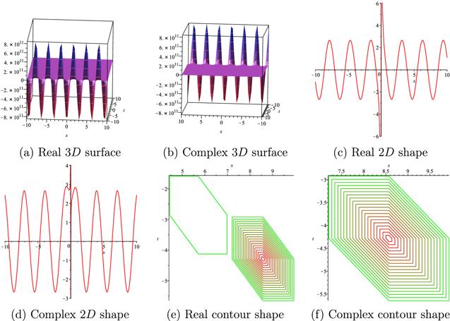
Figure 1. Graphical descriptions of the solution E11(x, t) under the values p = 2, q = 0.5, r = 2, $\mu$ = 1, $\delta$ = 3 and t = 0.01 for 2D graphics. |
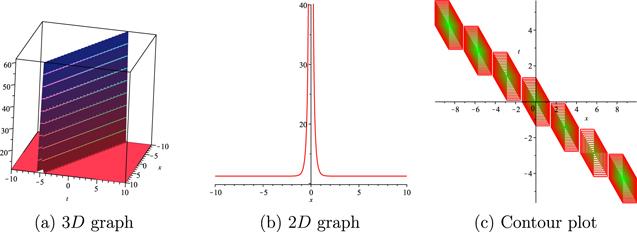
Figure 2. Graphical descriptions of the solution n11(x, t) under the values p = 2, q = 0.5, r = 2, $\mu$ = 1, $\delta$ = 3 and t = 0.01 for 2D graphics. |
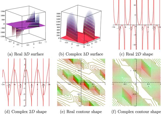
Figure 3. Graphical descriptions of the solution E13(x, t) when p = 2, q = 0.5, r = 2, $\mu$ = 2, $\delta$ = 2 and for 2D graphics t = 0.01. |
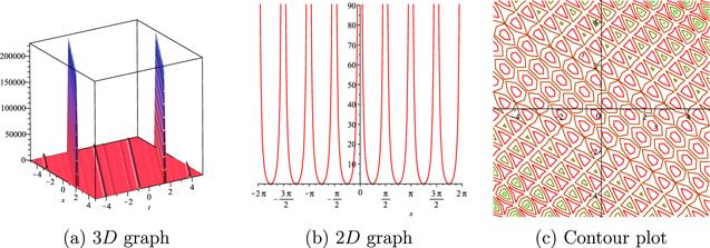
Figure 4. Graphical descriptions of the solution n13(x, t) when p = 2, q = 0.5, r = 2, $\mu$ = 2, $\delta$ = 2 and for 2D graphics t = 0.01. |
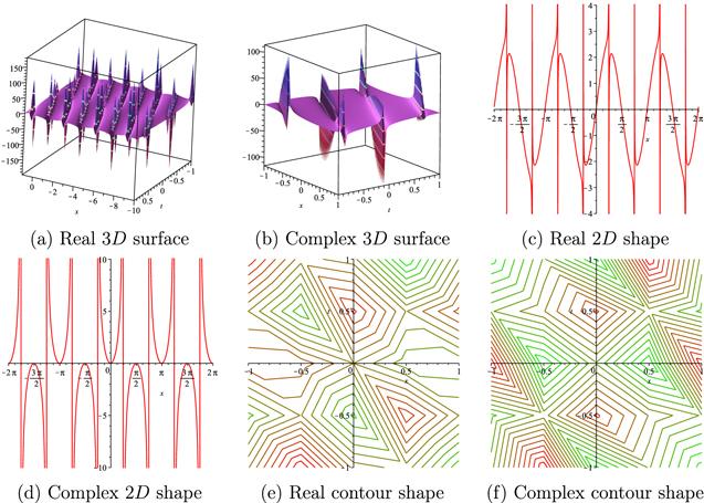
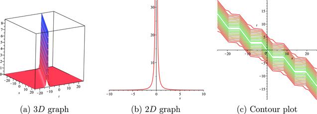
Figure 5. Graphical descriptions of the solution E14(x, t) when p = 2, q = 0.5, r = 2, $\mu$ = 2, $\delta$ = 2 and for 2D graphics t = 0.01. |
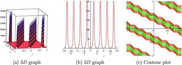
Figure 6. Graphical descriptions of the solution n14(x, t) when p = 2, q = 0.5, r = 2, $\mu$ = 2, $\delta$ = 2 and for 2D graphics t = 0.01. |
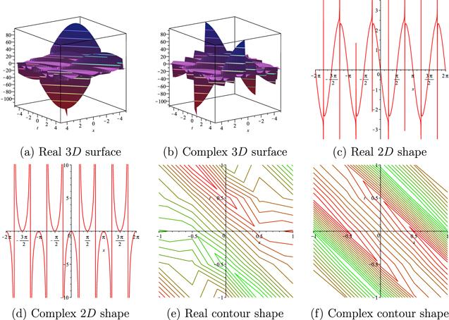
Figure 7. Graphical descriptions of the solution E23(x, t) when p = 2, q = 0.5, r = 2, $\mu$ = 2, $\delta$ = 2 and for 2D graphics t = 0.01. |
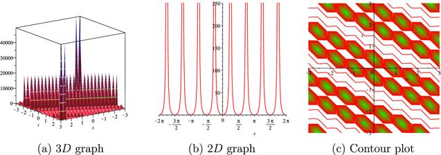
Figure 8. Graphical descriptions of the solution n23(x, t) when p = 2, q = 0.5, r = 2, $\mu$ = 2, $\delta$ = 2 and for 2D graphics t = 0.01. |
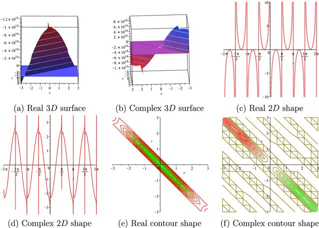
Figure 9. Graphical descriptions of the solution E24(x, t) when p = 2, q = 0.5, r = 2, $\mu$ = 2, $\delta$ = 2 and for 2D graphics t = 0.01. |
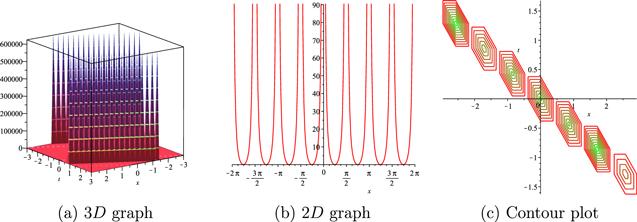
Figure 10. Graphical descriptions of the solution n24(x, t) when p = 2, q = 0.5, r = 2, $\mu$ = 2, $\delta$ = 2 and for 2D graphics t = 0.01. |

Figure 11. Graphical descriptions of the solution E45(x, t) when p = 2, q = 0.5, r = 2, $\mu$ = 2, $\delta$ = 2 and for 2D graphics t = 0.01. |
Figure 12. Graphical descriptions of the solution n45(x, t) when p = 2, q = 0.5, r = 2, $\mu$ = 2, $\delta$ = 2 and for 2D graphics t = 0.01. |
4. Conclusion
 -expansion approach to obtain the closed-form wave structures of the studied equation. Furthermore, this approach concerned new closed-form wave structures like rational, trigonometrical and hyperbolic function solutions. The techniques prescribed the well-designed systems for supervising various nonlinear wave equations with integer-order and also with fraction order arising in several applications of applied sciences. As can be seen from the above solution process, the modified $(G^{\prime} /G)$
  -expansion method is very effective for solving different types of NPDEs. Our results show that the structures of the obtained wave solutions are multifarious in nonlinear dynamic systems. In the near future, we will modify the algorithm presented here to deal with different NPDEs when their coefficients are variables, for exhaling nonautonomous wave solutions.