


1. Introduction
Nonlinear partial differential equations (NPDEs) play an important role in describing various natural phenomena arising in physics [1–3], chemistry [4, 5], biology medical [6, 7] and so on [8–11]. The theory of solitons is one of the most important topics and there have been many solutions available such as generalized hyperbolic-function method [12], asymptotic methods [13], exp(−φ(ξ)) method [14], Hirota bilinear method [15], Hirota method [16], sinh-Gordon function method [17] and so on [18–20]. In this paper, we mainly study the nonlinear strain wave equation in microstructured solids which is governed as [21, 22]:
$\begin{eqnarray}\begin{array}{l}{\varphi }_{tt}-{\varphi }_{xx}-\kappa {\lambda }_{1}{\left({\varphi }^{2}\right)}_{xx}-\alpha {\lambda }_{2}{\varphi }_{txx}+\varepsilon {\lambda }_{3}{\varphi }_{xxxx}\\ \,-\,\left(\varepsilon {\lambda }_{4}-{\alpha }^{2}{\lambda }_{7}\right){\varphi }_{ttxx}+\alpha \varepsilon \left({\lambda }_{5}{\varphi }_{txxxx}+{\lambda }_{6}{\varphi }_{tttxx}\right)=0,\end{array}\end{eqnarray}$
where $\kappa $ denotes elastic strains, $\varepsilon $ is the ratio between the microstructure size and the wavelength, $\alpha $ characterizes the influence of dissipation and ${\lambda }_{i}\left(i=1,2,\mathrm{...},5,6,7\right)$ are constants. The special case of $\alpha =0$ leads to the non dissipative form of the micro strain wave, which can be expressed as: $\begin{eqnarray}{\varphi }_{tt}-{\varphi }_{xx}-\kappa {\lambda }_{1}{\left({\varphi }^{2}\right)}_{xx}+\varepsilon {\lambda }_{3}{\varphi }_{xxxx}-\varepsilon {\lambda }_{4}{\varphi }_{ttxx}=0.\end{eqnarray}$
Recently, the fractional calculus and fractal calculus are the hot topics and have been widely used to model many complex problems involving in physics [23], filter [24–26], biological [27, 28], circuit [29, 30] and so on [31–33]. Inspired by recent research results on the fractional calculus, we extend the nonlinear strain wave equation into its time-space fractional form by applying the fractional calculus to equation (1.2 ) as:
$\begin{eqnarray}\begin{array}{l}\displaystyle \frac{{\partial }_{\hslash }^{2}}{\partial {t}^{2\eta }}\left(\varphi \right)-\displaystyle \frac{{\partial }_{\hslash }^{2}}{\partial {x}^{2\varsigma }}\left(\varphi \right)-\kappa {\lambda }_{1}\displaystyle \frac{{\partial }_{\hslash }^{2}}{\partial {x}^{2\varsigma }}\left({\varphi }^{2}\right)+\varepsilon {\lambda }_{3}\displaystyle \frac{{\partial }_{\hslash }^{4}}{\partial {x}^{4\varsigma }}\left(\varphi \right)\\ \,-\,\varepsilon {\lambda }_{4}\displaystyle \frac{{\partial }_{\hslash }^{2}}{\partial {t}^{2\eta }}\displaystyle \frac{{\partial }_{\hslash }^{2}}{\partial {x}^{2\varsigma }}\left(\varphi \right)=0.\end{array}\end{eqnarray}$
Among the above equation, $0\lt \eta \leqslant 1,$ $0\lt \varsigma \leqslant 1,$ $\tfrac{{\partial }_{\hslash }}{\partial {t}^{\eta }}$ and $\tfrac{{\partial }_{\hslash }}{\partial {x}^{\varsigma }}$ are the fractional derivatives with respect to $t$ and $x$ that defined as [34, 35]:
$\begin{eqnarray}\displaystyle \frac{{\partial }_{\hslash }}{\partial {t}^{\eta }}\left(\phi \left(x,{t}_{0}\right)\right)={\rm{\Gamma }}\left(1+\eta \right)\mathop{\mathrm{lim}}\limits_{\begin{array}{l}t-{t}_{0}={\rm{\Delta }}t\\ {\rm{\Delta }}t\ne 0\end{array}}\displaystyle \frac{\varphi \left(x,t\right)-\varphi \left(x,{t}_{0}\right)}{{\left(t-{t}_{0}\right)}^{\eta }},\end{eqnarray}$
$\begin{eqnarray}\displaystyle \frac{{\partial }_{\hslash }}{\partial {x}^{\varsigma }}\left(\phi \left({x}_{0},t\right)\right)={\rm{\Gamma }}\left(1+\varsigma \right)\mathop{\mathrm{lim}}\limits_{\begin{array}{l}x-{x}_{0}={\rm{\Delta }}x\\ {\rm{\Delta }}x\ne 0\end{array}}\displaystyle \frac{\varphi \left(x,t\right)-\varphi \left({x}_{0},t\right)}{{\left(x-{x}_{0}\right)}^{\varsigma }}.\end{eqnarray}$
And the following chain rules are given:
$\begin{eqnarray}\displaystyle \frac{{\partial }_{\hslash }^{2}}{\partial {t}^{2\eta }}=\displaystyle \frac{{\partial }_{\hslash }}{\partial {t}^{\eta }}\displaystyle \frac{{\partial }_{\hslash }}{\partial {t}^{\eta }},\end{eqnarray}$
$\begin{eqnarray}\displaystyle \frac{{\partial }_{\hslash }^{2}}{\partial {x}^{2\varsigma }}=\displaystyle \frac{{\partial }_{\hslash }}{\partial {x}^{\varsigma }}\displaystyle \frac{{\partial }_{\hslash }}{\partial {x}^{\varsigma }},\end{eqnarray}$
$\begin{eqnarray}\displaystyle \frac{{\partial }_{\hslash }}{\partial {x}^{\varsigma }}\displaystyle \frac{{\partial }_{\hslash }^{2}}{\partial {t}^{2\eta }}=\displaystyle \frac{{\partial }_{\hslash }}{\partial {x}^{\varsigma }}\displaystyle \frac{{\partial }_{\hslash }}{\partial {t}^{\eta }}\displaystyle \frac{{\partial }_{\hslash }}{\partial {t}^{\eta }}.\end{eqnarray}$
For the special case $\eta =\varsigma =1,$ the fractional nonlinear strain wave equation of equation (1.3 ) converts into the classic strain wave equation as shown in equation (1.2 ).
2. The two-scale transform
Suppose there is the following time-space fractional equation:
$\begin{eqnarray}\displaystyle \frac{{\partial }_{\hslash }\varphi }{\partial {t}^{\eta }}+\displaystyle \frac{{\partial }_{\hslash }\varphi }{\partial {x}^{\varsigma }}+F\left(\varphi \right)=0.\end{eqnarray}$
The definitions of the fractional derivatives are given in equations (1.4 ) and (1.5 ).
We introduce the two-scale transforms as:
$\begin{eqnarray}T={t}^{\eta },\end{eqnarray}$
$\begin{eqnarray}X={x}^{\varsigma }.\end{eqnarray}$
Applying above transforms for equation (2.1 ), then equation (2.1 ) can be converted into its partner as:
$\begin{eqnarray}\displaystyle \frac{\partial \varphi }{\partial T}+\displaystyle \frac{\partial \varphi }{\partial X}+F(\varphi )=0.\end{eqnarray}$
Thus equation (2.4 ) can be solved by many classical methods such as Homotopy perturbation method, variational iteration method, Taylor series method, Exp-function method and so on.
3. Variational formulation
Considering the following two-scale transforms:
$\begin{eqnarray}T={t}^{\eta },\end{eqnarray}$
$\begin{eqnarray}X={x}^{\varsigma }.\end{eqnarray}$
Then we can convert equation (1.3 ) into the following form:
$\begin{eqnarray}{\varphi }_{TT}-{\varphi }_{XX}-\kappa {\lambda }_{1}{\left({\varphi }^{2}\right)}_{XX}+\varepsilon {\lambda }_{3}{\varphi }_{XXXX}-\varepsilon {\lambda }_{4}{\varphi }_{TTXX}=0.\end{eqnarray}$
Applying the following transformation for equation (3.3 ):
$\begin{eqnarray}\varphi \left(X,T\right)=\varphi \left({\rm{\Xi }}\right),{\rm{\Xi }}=X-vT+{{\rm{\Xi }}}_{0}.\end{eqnarray}$
By bringing equation (3.4 ) into (3.3 ), it gives:
$\begin{eqnarray}\begin{array}{l}\varepsilon \left({\lambda }_{3}-{\lambda }_{4}{v}^{2}\right){\varphi }^{\left(4\right)}\left({\rm{\Xi }}\right)+\left({v}^{2}-1\right)\varphi ^{\prime\prime} \left({\rm{\Xi }}\right)\\ \,-\,2\kappa {\lambda }_{1}\left[{\left(\varphi ^{\prime} \left({\rm{\Xi }}\right)\right)}^{2}+\varphi \left({\rm{\Xi }}\right)\varphi ^{\prime\prime} \left({\rm{\Xi }}\right)\right]=0.\end{array}\end{eqnarray}$
Take a integration for above equation and neglect the integration constant, we have:
$\begin{eqnarray}\varepsilon \left({\lambda }_{3}-{\lambda }_{4}{v}^{2}\right){\varphi }^{\left(3\right)}\left({\rm{\Xi }}\right)+\left({v}^{2}-2\kappa {\lambda }_{1}\varphi \left({\rm{\Xi }}\right)-1\right)\varphi ^{\prime} \left({\rm{\Xi }}\right)=0.\end{eqnarray}$
Take the same operation for equation (3.6 ) yields:
$\begin{eqnarray}\varepsilon \left({\lambda }_{3}-{\lambda }_{4}{v}^{2}\right)\varphi ^{\prime\prime} \left({\rm{\Xi }}\right)-\kappa {\lambda }_{1}{\varphi }^{2}\left({\rm{\Xi }}\right)+\left({v}^{2}-1\right)\varphi \left({\rm{\Xi }}\right)=0.\end{eqnarray}$
Using the semi-inverse method [38–50], the variational formulation of equation (3.7 ) can be easily obtained as:
$\begin{eqnarray}\begin{array}{l}J\left(\varphi \right)=\displaystyle \int \left\{-\displaystyle \frac{1}{2}\varepsilon \left({\lambda }_{3}-{\lambda }_{4}{v}^{2}\right){\left(\varphi ^{\prime} \right)}^{2}-\displaystyle \frac{1}{3}\kappa {\lambda }_{1}{\varphi }^{3}\right.\\ \,\,\,+\,\left.\displaystyle \frac{1}{2}\left({v}^{2}-1\right){\varphi }^{2}\right\}{\rm{d}}{\rm{\Xi }},\end{array}\end{eqnarray}$
which can be re-written as: $\begin{eqnarray}J\left(\varphi \right)=\displaystyle \int \left\{\psi {\left(\varphi ^{\prime} \right)}^{2}-\delta {\varphi }^{3}+\sigma {\varphi }^{2}\right\}{\rm{d}}{\rm{\Xi }},\end{eqnarray}$
where $\psi =-\tfrac{1}{2}\varepsilon \left({\lambda }_{3}-{\lambda }_{4}{v}^{2}\right),$ $\delta =\tfrac{1}{3}\kappa {\lambda }_{1},$ $\sigma =\tfrac{1}{2}\left({v}^{2}-1\right).$By comparing equations (3.9 ) and (3.7 ), it can be seen that the order of the differential equation has been reduced by the variational method.
4. Solitary wave solutions
In this section, we aim to seek the solitary solution of equation (1.3 ) by the variational theory. According to He’s variational method [51–53], we suppose the solution of equation (3.7 ) with the following form:4.1 ) into (3.9 ), it yields:
$\begin{eqnarray}\varphi =p\text{sec}{{\rm{h}}}^{2}\left(q{\rm{\Xi }}\right),q\gt 0,\end{eqnarray}$
where $p$ and $q$ are unknown constants that can be determined later. Now we substitute equation ( $\begin{eqnarray}\begin{array}{l}J\left(p,q\right)=\displaystyle {\int }_{0}^{\infty }\left\{\psi {\left(\varphi ^{\prime} \right)}^{2}-\delta {\varphi }^{3}+\sigma {\varphi }^{2}\right\}{\rm{d}}{\rm{\Xi }}\\ \,\,\,\,=\,\displaystyle {\int }_{0}^{\infty }\left\{4\psi {p}^{2}{q}^{2}\text{sec}{{\rm{h}}}^{4}(q{\rm{\Xi }}){\tanh }^{2}(q{\rm{\Xi }})\right.\\ \,\,\,\,-\,\left.\delta {p}^{3}\text{sec}{{\rm{h}}}^{6}(q{\rm{\Xi }})+\sigma {p}^{2}\text{sec}{{\rm{h}}}^{4}(q{\rm{\Xi }})\right\}{\rm{d}}{\rm{\Xi }}\\ \,\,\,\,=\,\displaystyle {\int }_{0}^{\infty }\left\{4\psi {p}^{2}q\text{sec}{{\rm{h}}}^{4}(\omega ){\tanh }^{2}(\omega )\right.\\ \,\,\,\,-\,\left.\displaystyle \frac{\delta {p}^{3}}{q}\text{sec}{{\rm{h}}}^{6}(\omega )+\displaystyle \frac{\sigma {p}^{2}}{q}\text{sec}{{\rm{h}}}^{4}(\omega )\right\}{\rm{d}}\omega \\ \,\,\,\,=\,4\psi {p}^{2}{q}^{2}\displaystyle {\int }_{0}^{\infty }\text{sec}{{\rm{h}}}^{4}(\omega ){\tanh }^{2}(\omega ){\rm{d}}\omega \\ \,\,\,\,-\,\displaystyle \frac{\delta {p}^{3}}{q}\displaystyle {\int }_{0}^{\infty }\text{sec}{{\rm{h}}}^{6}(\omega ){\rm{d}}\omega +\displaystyle \frac{\sigma {p}^{2}}{q}\displaystyle {\int }_{0}^{\infty }\text{sec}{{\rm{h}}}^{4}(\omega ){\rm{d}}\omega \\ \,\,\,\,=\,\displaystyle \frac{2{p}^{2}\left(5\sigma -4\delta p+4\psi {q}^{2}\right)}{15q}.\end{array}\end{eqnarray}$
The following results can be obtained by calculating equations (4.3 ) and (4.4 ):
$\begin{eqnarray}\displaystyle \frac{4p\left(5\sigma -6\delta p+4\psi {q}^{2}\right)}{15q}=0,\end{eqnarray}$
$\begin{eqnarray}\displaystyle \frac{2{p}^{2}\left(-5\sigma +4\delta p+4\psi {q}^{2}\right)}{15{q}^{2}}=0,\end{eqnarray}$
where $\begin{eqnarray}\psi =-\displaystyle \frac{1}{2}\varepsilon \left({\lambda }_{3}-{\lambda }_{4}{v}^{2}\right),\delta =\displaystyle \frac{1}{3}\kappa {\lambda }_{1},\sigma =\displaystyle \frac{1}{2}\left({v}^{2}-1\right).\end{eqnarray}$
Solving equations (4.5 ) and (4.6 ), we have:
$\begin{eqnarray}p=\displaystyle \frac{\sigma }{\delta },\end{eqnarray}$
$\begin{eqnarray}q=\displaystyle \frac{1}{2}\sqrt{\displaystyle \frac{\sigma }{\psi }}.\end{eqnarray}$
Substituting equation (4.7 ) into the above formulas, the unknown constants $p$ and $q$ can be determined as:
$\begin{eqnarray}p=\displaystyle \frac{3\left({v}^{2}-1\right)}{\kappa {\lambda }_{1}},\end{eqnarray}$
$\begin{eqnarray}q=\displaystyle \frac{1}{2}\sqrt{\displaystyle \frac{{v}^{2}-1}{\varepsilon \left({\lambda }_{4}{v}^{2}-{\lambda }_{3}\right)}}.\end{eqnarray}$
With this, the solution of equation (3.7 ) can be obtained as:
$\begin{eqnarray}\varphi \left({\rm{\Xi }}\right)=\displaystyle \frac{3\left({v}^{2}-1\right)}{\kappa {\lambda }_{1}}\text{sec}{{\rm{h}}}^{2}\left(\displaystyle \frac{1}{2}\sqrt{\displaystyle \frac{{v}^{2}-1}{\varepsilon \left({\lambda }_{4}{v}^{2}-{\lambda }_{3}\right)}}{\rm{\Xi }}\right).\end{eqnarray}$
Then we can get the solitary wave solution of equation (3.3 ) via equation (3.4 ) as:
$\begin{eqnarray}\begin{array}{l}\varphi \left(X,T\right)=\displaystyle \frac{3\left({v}^{2}-1\right)}{\kappa {\lambda }_{1}}\text{sec}{{\rm{h}}}^{2}\left(\displaystyle \frac{1}{2}\sqrt{\displaystyle \frac{{v}^{2}-1}{\varepsilon \left({\lambda }_{4}{v}^{2}-{\lambda }_{3}\right)}}\right.\\ \,\,\,\,\,\times \,\left.\left(X-vT+{{\rm{\Xi }}}_{0}\right)\right).\end{array}\end{eqnarray}$
Thus the solitary solution of equation (1.3 ) can be obtained by using the two-scale transforms of equations (3.1 ) and (3.2 ) as:1.2 ).
$\begin{eqnarray}\begin{array}{l}\varphi \left(x,t\right)=\displaystyle \frac{3\left({v}^{2}-1\right)}{\kappa {\lambda }_{1}}\text{sec}{{\rm{h}}}^{2}\left(\displaystyle \frac{1}{2}\sqrt{\displaystyle \frac{{v}^{2}-1}{\varepsilon \left({\lambda }_{4}{v}^{2}-{\lambda }_{3}\right)}}\right.\\ \,\,\,\,\times \,\left.\left({x}^{\varsigma }-v{t}^{\eta }+{{\rm{\Xi }}}_{0}\right)\right).\end{array}\end{eqnarray}$
When $\eta =\varsigma =1,$ the above solution becomes the solitary wave solution of the classic strain wave equation as shown in equation (It must be pointed out that we can obtain other soliton solutions by setting $\varphi \left({\rm{\Xi }}\right)=p\csc {\rm{h}}\left(q{\rm{\Xi }}\right),$ $\varphi \left({\rm{\Xi }}\right)=p\,\tanh \left(q{\rm{\Xi }}\right)$ and $\varphi \left({\rm{\Xi }}\right)=p\,\coth \left(q{\rm{\Xi }}\right)$ using the same method.
5. Periodic wave solutions
In this section, we will try to obtain the periodic wave solution of equation (1.3 ). In the light of He’s variational method [54–56], the periodic solution of equation (3.7 ) is assumed to take the form as:
$\begin{eqnarray}\varphi \left({\rm{\Xi }}\right)={\rm{\Lambda }}\,\cos \left(\varpi {\rm{\Xi }}\right),\varpi \gt 0,\end{eqnarray}$
Substituting equation (5.1 ) into (3.8 ) yields:
$\begin{eqnarray}\begin{array}{l}J\left(\varphi \right)=\displaystyle {\int }_{0}^{\tfrac{T}{4}}\left\{-\displaystyle \frac{1}{2}\varepsilon \left({\lambda }_{3}-{\lambda }_{4}{v}^{2}\right){\left(\varphi ^{\prime} \right)}^{2}-\displaystyle \frac{1}{3}\kappa {\lambda }_{1}{\varphi }^{3}\right.\\ \,\,\,+\,\left.\displaystyle \frac{1}{2}\left({v}^{2}-1\right){\varphi }^{2}\right\}{\rm{d}}{\rm{\Xi }}\\ \,\,\,=\displaystyle {\int }_{0}^{\tfrac{T}{4}}\left\{-\displaystyle \frac{1}{2}\varepsilon \left({\lambda }_{3}-{\lambda }_{4}{v}^{2}\right){\left[-{\rm{\Lambda }}\varpi \sin \left(\varpi {\rm{\Xi }}\right)\right]}^{2}\right.\\ \,\,\,-\,\displaystyle \frac{1}{3}\kappa {\lambda }_{1}{\left[{\rm{\Lambda }}\cos \left(\varpi {\rm{\Xi }}\right)\right]}^{3}+\displaystyle \frac{1}{2}\left({v}^{2}-1\right)\\ \,\,\,\times \,\left.{\left[{\rm{\Lambda }}\cos \left(\varpi {\rm{\Xi }}\right)\right]}^{2}\right\}{\rm{d}}{\rm{\Xi }}\\ \,\,=\displaystyle \frac{1}{\varpi }\displaystyle {\int }_{0}^{\tfrac{\pi }{2}}\left\{-\displaystyle \frac{1}{2}\varepsilon \left({\lambda }_{3}-{\lambda }_{4}{v}^{2}\right){\left[-{\rm{\Lambda }}\varpi \sin \left({\rm{\Pi }}\right)\right]}^{2}\right.\\ \,\,\,-\,\displaystyle \frac{1}{3}\kappa {\lambda }_{1}{\left[{\rm{\Lambda }}\cos \left({\rm{\Pi }}\right)\right]}^{3}+\displaystyle \frac{1}{2}\left({v}^{2}-1\right)\\ \,\,\,\times \,\left.{\left[{\rm{\Lambda }}\cos \left({\rm{\Pi }}\right)\right]}^{2}\right\}{\rm{d}}{\rm{\Pi }}.\end{array}\end{eqnarray}$
According to He’s variational method [54–57], we have:
$\begin{eqnarray}\displaystyle \frac{{\rm{d}}J}{{\rm{d}}{\rm{\Lambda }}}=0,\end{eqnarray}$
which leads to: $\begin{eqnarray}\begin{array}{l}\displaystyle \frac{{\rm{d}}J\left(\varphi \right)}{{\rm{d}}{\rm{\Lambda }}}=\displaystyle \frac{{\rm{d}}}{{\rm{d}}{\rm{\Lambda }}}\displaystyle {\int }_{0}^{\tfrac{T}{4}}\left\{-\displaystyle \frac{1}{2}\varepsilon \left({\lambda }_{3}-{\lambda }_{4}{v}^{2}\right){\left(\varphi ^{\prime} \right)}^{2}-\displaystyle \frac{1}{3}\kappa {\lambda }_{1}{\varphi }^{3}\right.\\ \,\,\,\,+\,\left.\displaystyle \frac{1}{2}\left({v}^{2}-1\right){\varphi }^{2}\right\}{\rm{d}}{\rm{\Xi }}\\ \,\,\,=\,\displaystyle \frac{{\rm{d}}}{{\rm{d}}{\rm{\Lambda }}}\displaystyle {\int }_{0}^{\tfrac{T}{4}}\left\{-\displaystyle \frac{1}{2}\varepsilon \left({\lambda }_{3}-{\lambda }_{4}{v}^{2}\right){\left[-{\rm{\Lambda }}\varpi \sin \left(\varpi {\rm{\Xi }}\right)\right]}^{2}\right.\\ \,\,\,\,-\,\displaystyle \frac{1}{3}\kappa {\lambda }_{1}{\left[{\rm{\Lambda }}\cos \left(\varpi {\rm{\Xi }}\right)\right]}^{3}+\displaystyle \frac{1}{2}\left({v}^{2}-1\right)\\ \,\,\,\,\times \,\left.{\left[{\rm{\Lambda }}\cos \left(\varpi {\rm{\Xi }}\right)\right]}^{2}\right\}{\rm{d}}{\rm{\Xi }}\\ \,\,\,=\,\displaystyle \frac{1}{\varpi }\displaystyle \frac{{\rm{d}}}{{\rm{d}}{\rm{\Lambda }}}\displaystyle {\int }_{0}^{\tfrac{\pi }{2}}\left\{-\displaystyle \frac{1}{2}\varepsilon \left({\lambda }_{3}-{\lambda }_{4}{v}^{2}\right){\left[-{\rm{\Lambda }}\varpi \sin \left({\rm{\Pi }}\right)\right]}^{2}\right.\\ \,\,\,\,-\,\displaystyle \frac{1}{3}\kappa {\lambda }_{1}{\left[{\rm{\Lambda }}\cos \left({\rm{\Pi }}\right)\right]}^{3}+\displaystyle \frac{1}{2}\left({v}^{2}-1\right)\\ \,\,\,\,\times \,\left.{\left[{\rm{\Lambda }}\cos \left({\rm{\Pi }}\right)\right]}^{2}\right\}{\rm{d}}{\rm{\Pi }}\\ \,\,\,=\,\displaystyle \frac{1}{\varpi }\displaystyle {\int }_{0}^{\tfrac{\pi }{2}}\left\{-\varepsilon \left({\lambda }_{3}-{\lambda }_{4}{v}^{2}\right){\rm{\Lambda }}{\varpi }^{2}{\sin }^{2}\left({\rm{\Pi }}\right)\right.\\ \,\,\,\,-\,\left.\kappa {\lambda }_{1}{{\rm{\Lambda }}}^{2}{\cos }^{3}\left({\rm{\Pi }}\right)+\left({v}^{2}-1\right){\rm{\Lambda }}{\cos }^{2}\left({\rm{\Pi }}\right)\right\}{\rm{d}}{\rm{\Pi }}\\ \,\,\,=\,0.\end{array}\end{eqnarray}$
In the view of equation (5.4 ), we have:
$\begin{eqnarray}{\varpi }^{2}=\displaystyle \frac{\displaystyle {\int }_{0}^{\tfrac{\pi }{2}}\left\{-\kappa {\lambda }_{1}{{\rm{\Lambda }}}^{2}{\cos }^{3}\left({\rm{\Pi }}\right)+\left({v}^{2}-1\right){\rm{\Lambda }}{\cos }^{2}\left({\rm{\Pi }}\right)\right\}{\rm{d}}{\rm{\Pi }}}{\displaystyle {\int }_{0}^{\tfrac{\pi }{2}}\left\{\varepsilon \left({\lambda }_{3}-{\lambda }_{4}{v}^{2}\right){\rm{\Lambda }}{\sin }^{2}\left({\rm{\Pi }}\right)\right\}{\rm{d}}{\rm{\Pi }}}.\end{eqnarray}$
Calculating above equation, we obtain:
$\begin{eqnarray}\varpi =\sqrt{-\displaystyle \frac{8{\rm{\Lambda }}\kappa {\lambda }_{1}}{3\varepsilon \left({\lambda }_{3}-{\lambda }_{4}{v}^{2}\right)\pi }+\displaystyle \frac{\left({v}^{2}-1\right)}{\varepsilon \left({\lambda }_{3}-{\lambda }_{4}{v}^{2}\right)}}\gt 0.\end{eqnarray}$
Taking above equation into equation (5.1 ), we have:
$\begin{eqnarray}\varphi \left({\rm{\Xi }}\right)={\rm{\Lambda }}\,\cos \left(\sqrt{-\displaystyle \frac{8{\rm{\Lambda }}\kappa {\lambda }_{1}}{3\varepsilon \left({\lambda }_{3}-{\lambda }_{4}{v}^{2}\right)\pi }+\displaystyle \frac{\left({v}^{2}-1\right)}{\varepsilon \left({\lambda }_{3}-{\lambda }_{4}{v}^{2}\right)}}{\rm{\Xi }}\right).\end{eqnarray}$
Therefore, we can get the periodic wave solution of equation (3.3 ) via equation (3.4 ) as:
$\begin{eqnarray}\begin{array}{l}\varphi \left(X,T\right)={\rm{\Lambda }}\,\cos \left(\sqrt{-\displaystyle \frac{8{\rm{\Lambda }}\kappa {\lambda }_{1}}{3\varepsilon \left({\lambda }_{3}-{\lambda }_{4}{v}^{2}\right)\pi }+\displaystyle \frac{\left({v}^{2}-1\right)}{\varepsilon \left({\lambda }_{3}-{\lambda }_{4}{v}^{2}\right)}}\right.\\ \,\,\,\,\,\times \,\left.\left(X-vT+{{\rm{\Xi }}}_{0}\right)\right).\end{array}\end{eqnarray}$
With the help of the the two-scale transforms of equations (3.1 ) and (3.2 ), the periodic wave solution of equation (1.3 ) can be approximated as:1.3 ).
$\begin{eqnarray}\begin{array}{l}\phi \left(x,t\right)={\rm{\Lambda }}\,\cos \left(\sqrt{-\displaystyle \frac{8{\rm{\Lambda }}\kappa {\lambda }_{1}}{3\varepsilon \left({\lambda }_{3}-{\lambda }_{4}{v}^{2}\right)\pi }+\displaystyle \frac{\left({v}^{2}-1\right)}{\varepsilon \left({\lambda }_{3}-{\lambda }_{4}{v}^{2}\right)}}\right.\\ \,\,\,\times \,\left.\left({x}^{\varsigma }-v{t}^{\eta }+{{\rm{\Xi }}}_{0}\right)\right),\end{array}\end{eqnarray}$
which is the exact periodic wave solution of the fractional strain wave equation in microstructured solids in equation (When $\eta =\varsigma =1,$ equation (5.9 ) becomes the periodic wave solution of the classic strain wave equation as shown in equation (1.2 ).
It must be noted that we can obtain another periodic wave solution by assuming $\varphi \left({\rm{\Xi }}\right)={\rm{\Lambda }}\,\sin \left(\varpi {\rm{\Xi }}\right)$ via the same method.
6. One example
In this section, we use an example to illustrate the effectiveness and reliability of the proposed method. Here we set ${\lambda }_{1}=1,$ ${\lambda }_{3}=2,$ ${\lambda }_{4}=1,$ $\kappa =2,$ $\varepsilon =1,$ $v=2,$ then equation (1.3 ) can be written as:
$\begin{eqnarray}\begin{array}{l}\displaystyle \frac{{\partial }_{\hslash }^{2}}{\partial {t}^{2\eta }}\left(\varphi \right)-\displaystyle \frac{{\partial }_{\hslash }^{2}}{\partial {x}^{2\varsigma }}\left(\varphi \right)-2\displaystyle \frac{{\partial }_{\hslash }^{2}}{\partial {x}^{2\varsigma }}\left({\varphi }^{2}\right)+2\displaystyle \frac{{\partial }_{\hslash }^{4}}{\partial {x}^{4\varsigma }}\left(\varphi \right)\\ \,-\,\displaystyle \frac{{\partial }_{\hslash }^{2}}{\partial {t}^{2\eta }}\displaystyle \frac{{\partial }_{\hslash }^{2}}{\partial {x}^{2\varsigma }}\left(\varphi \right)=0.\end{array}\end{eqnarray}$
6.1. The solitary wave solution
According to equation (4.14 ), we can get the solitary wave solution of equation (6.1 ) as:
$\begin{eqnarray}\varphi \left(x,t\right)=\displaystyle \frac{9}{2}\text{sec}{{\rm{h}}}^{2}\left(\displaystyle \frac{1}{2}\sqrt{\displaystyle \frac{3}{2}}\left({x}^{\varsigma }-2{t}^{\eta }+{{\rm{\Xi }}}_{0}\right)\right).\end{eqnarray}$
Then we plot the behavior of equation (6.2 ) with different fractional orders of $\eta $ and $\varsigma $ in figure 1.
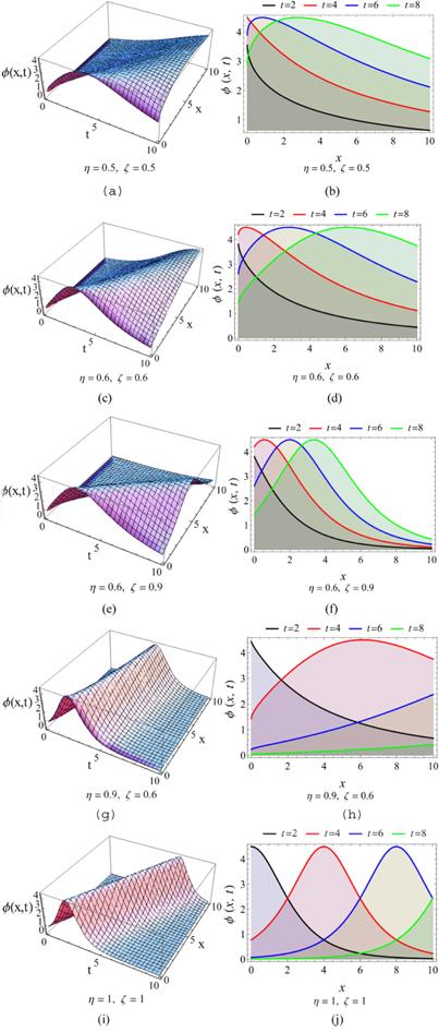
Figure 1. The behavior of equation ( |
Form the 3D and 2D plots of equation (6.2 ) with different fractional orders $\eta $ and $\varsigma ,$ it can be found that the smaller the fractional orders are, the slower the solitary wave changes. In addition, when the $\eta \gg \varsigma ,$ the peak of solitary wave tends to be parallel to x-direction. On the contrary, it tends to the vertical x-direction. When $\eta =\varsigma =1,$ the plots in figures 1(i)–(j) are perfect bright solitary waves, which are the solitary waves of the classic strain wave equation.
6.2. The periodic wave solution
For ${\rm{\Lambda }}=4,$ the periodic wave solution of of equation (6.1 ) can be obtained by equation (5.9 ) as:
$\begin{eqnarray}\varphi \left(x,t\right)=4\,\cos \left(\sqrt{\displaystyle \frac{64-9\pi }{6\pi }}\left({x}^{\varsigma }-2{t}^{\eta }+{{\rm{\Xi }}}_{0}\right)\right).\end{eqnarray}$
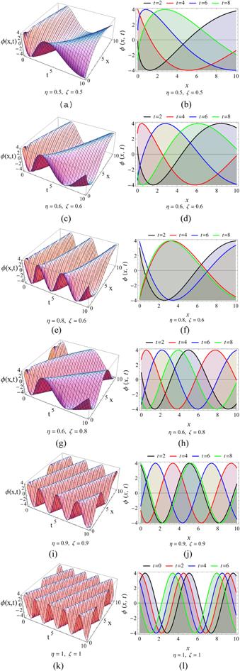
Then we plot the behaviors of equation (6.3 ) with different fractional orders of $\eta $ and $\varsigma $ in figure 2.
Figure 2. The behaviors of equation ( |
Figure 2 presents the periodic waves obtained by equation (6.3 ), we can observe that when $\eta \lt 1$ and $\varsigma \lt 1,$ the contours are kinky periodic waves. And the smaller the fractional orders are, the larger the period is. Besides, when the $\eta \gt $ $\varsigma ,$ the propagation direction of periodic wave tends to be perpendicular to x-direction. On the contrary, it tends to be parallel to x-direction. When $\eta =\varsigma =1,$ the plots in figures 2(k), (l) are perfect periodic waves, which are the periodic waves of the classic strain wave equation.
7. Conclusion
In this paper, He’s variational method together with the two-scale transform are used to find the solitary and periodic wave solutions of the time-space fractional strain wave equation in microstructured solids. The main advantage of variational approach is that it can reduce the order of differential equation and make the equation more simple. One example is given to verify the applicability and effectiveness of the method through the 3D and 2D contours. It shows that the variational method is simple and straightforward, and can avoid the tedious calculation process, which is expected to open some new perspectives towards the study of fractional NPDEs arsing in physics.