Welcome to visit Communications in Theoretical Physics,
Mathematical Physics

Magnetohydrodynamic flow and heat transfer of a hybrid nanofluid over a rotating disk by considering Arrhenius energy

  • M Gnaneswara Reddy 1 ,
  • Naveen Kumar R 2 ,
  • B C Prasannakumara 2 ,
  • N G Rudraswamy 3 ,
  • K Ganesh Kumar , 1
Expand
  • 1Department of Mathematics, Acharya Nagarjuna University Campus, Ongole-523 001, India
  • 2Department of Studies and Research in Mathematics, Davangere University, Shivagangothri, Davangere-577007, Karnataka, India
  • 3Department of Mathematics, P.C. Jabin Science Collage, Hubballi-580031, India

Received date: 2020-08-13

  Revised date: 2020-12-29

  Accepted date: 2021-01-11

  Online published: 2021-04-12

Copyright

© 2021 Institute of Theoretical Physics CAS, Chinese Physical Society and IOP Publishing

Abstract

This research work explores the effect of hybrid nanoparticles on the flow over a rotating disk by using an activation energy model. Here, we considered molybdenum disulfide and ferro sulfate as nanoparticles suspended in base fluid water. The magnetic field is pragmatic normal to the hybrid nanofluid flow direction. The derived nonlinear ordinary differential equations are non-dimensionalized and worked out numerically with the help of Maple software by the RKF-45 method. The scientific results for a non-dimensionalized equation are presented for both nanoparticle and hybrid nanoparticle case. Accoutrements of various predominant restrictions on flow and thermal fields are scanned. Computation estimation for friction factor, local Nusselt number and Sherwood number are also executed. Results reveal that the reduction of the heat transfer rate is greater in hybrid nanoparticles when compared to nanoparticles for increasing values of Eckert Number and the thermal field enhances for the enhanced values of volume fraction.

Cite this article

M Gnaneswara Reddy , Naveen Kumar R , B C Prasannakumara , N G Rudraswamy , K Ganesh Kumar . Magnetohydrodynamic flow and heat transfer of a hybrid nanofluid over a rotating disk by considering Arrhenius energy[J]. Communications in Theoretical Physics, 2021 , 73(4) : 045002 . DOI: 10.1088/1572-9494/abdaa5

Nomenclature

$\left(u,v,w\right)$

Velocity components in $\left({{\rm{ms}}}^{-1}\right)$

$f^{\prime} (\eta )$

Radial velocity

$f(\eta )$

Axial velocity

$g(\eta )$

Tangential velocity

$k$

Thermal conductivity $({{\rm{Wm}}}^{-1}{{\rm{K}}}^{-1})$

$Pr$

Prandtl number

$A$

Stretching parameter

${j}_{{\rm{w}}}$

Mass flux

$(\rho {C}_{{p}})$

Heat capacitance $({\mathrm{kg}{\rm{m}}}^{-1}{{\rm{s}}}^{-2}{{\rm{K}}}^{-1})$

$T$

Fluid temperature

$K$

Permeability

$C$

Fluid concentration

${k}_{{\rm{r}}}^{2}$

Reaction rate $\left({{\rm{s}}}^{-1}\right)$

${E}_{{\rm{a}}}$

Activation energy

$E$

Non-dimensional activation energy

${k}^{* }$

Boltzmann constant $({{\rm{JK}}}^{-1})$

${a}_{1}$

Stretching constant

$P$

Pressure

${C}_{{\rm{f}}}$

Skin friction coefficient

${Re}$

Reynolds number

$Sc$

Schmidt number

$Ec$

Eckert number

$D$

Mass diffusivity $({{\rm{m}}}^{2}{{\rm{s}}}^{-1})$

$M$

Magnetic parameter

${\tau }_{{\rm{wt}}}$

Radial stress

${q}_{{\rm{w}}}$

Heat flux

$Sh$

Sherwood number,

$Nu$

Nusselt number

${B}_{0}$

Strength of magnetic field

${\tau }_{{\rm{w}}\phi }$

Transverse shear stress

Greek symbols
$\theta $

Non-dimensional temperature

$\sigma $

Electrical conductivity $\left({\rm{k}}{{\rm{g}}}^{-1}{{\rm{m}}}^{-3}{{\rm{s}}}^{3}{{\rm{A}}}^{2}\right)$

$\eta $

Transformed coordinate

${\varnothing }_{1},{\varnothing }_{2}$

Volume concentration

${\rm{\Omega }}$

Constant angular velocity $\left({{\rm{s}}}^{-1}\right)$

$\nu $

Kinematic viscosity $({{\rm{m}}}^{2}{{\rm{s}}}^{-1})$

$\varepsilon $

Pressure parameter

$\delta $

Temperature difference

$\mu $

Dynamic viscosity $({\rm{kg}}\,{{\rm{s}}}^{-1}{{\rm{m}}}^{-1})$

$\rho $

Density $({{\rm{kgm}}}^{-3})$

Subscript
${\rm{f}}$

Fluid

${\rm{bf}}$

Base fluid

${\rm{hnf}}$

Hybrid nanofluid

${{\rm{s}}}_{1},{{\rm{s}}}_{2}$

Solid particle

$\infty $

Ambient

${\rm{w}}$

Surface

1. Introduction

In the year 1889, Sweden's Nobel laureate Arrhenius embarked upon a theory encompassing the reaction rate of numerous chemical processes. The theory averred the relationship between temperature and reaction rate in an equation form termed the Arrhenius equation. He stated that the minimum energy required to begin a chemical reaction is called the activation energy. Later, the term was coined as Arrhenius activation energy. Furthermore, the nature of Arrhenius activation energy was re-examined by Menzinger and Wolfgang [1]. Jensen [2] scrutinized the contemporary use of the Arrhenius equation and activation energy through ICs. Hayat et al [3] addressed the influence of activation energy in the flow of dyadic chemically reactive third-grade fluid through a rotating disk. Khan et al [4] exhibited the influence of dyadic chemical reaction and Arrhenius activation energy with second-law scrutiny on nanofluid flow. Salahuddin et al [5] examined the inner energy change and stable-state 3D change in visco-elastic fluid flow in revolving state with added convective boundary conditions. The impact of Arrhenius activation energy on tangent hyperbolic fluid flow above an impelling stretched surface with zero mass-flux conditions was revealed by Kumar et al [6]. Khan et al [7] calculated the effect of Arrhenius activation energy on chemically reactive rotating flow subject to heat source and nonlinear heat flux. Asma et al [8] numerically examined the magnetohydrodynamic (MHD) flow of nanofluid due to a rotating disk with the effect of activation energy and chemical reaction.
MHD flow has a wide range of applications in engineering, geophysics, astrophysics, the study of earthquakes, aerospace engineering and biological fields. Ramzan et al [9] used Eyring–Powell nanofluid to illustrate MHD flow, taking account of chemical reactions. Zeeshan et al [10] scrutinized the MHD Couette–Poiseuille nanofluid flow by considering activation energy along with the chemical reaction. Stagnation-point flow and the effect of Newtonian heating over the surface of a nanofluid were investigated by Hakeem et al [11]. Lu et al [12] scrutinized the MHD flow with the help of Carreau nanofluid by applying zero mass-flux condition. Khan et al [13] considered 3D flow over a two-directional stretching sheet by using the Carreau rheological model. In researching magnetic effect, heat generation/absorption is taken into the account. The outcome of the research revealed that the velocity is dependent on Hartmann number. Reddy and Sandeep [14] explained the phenomena of MHD flow of Carreau nanofluid through the analysis of the different effects.
The fluid flow over a surface of rotating disks has attracted tremendous interest from scientists due to its several technical and aerospace applications. Greater effort from researchers is required in order to discover the hidden properties of rotating disks. This is because the fluid flow conduction through rotating disks is not only of speculative interest, but has practical significance in the use of medical equipment, gas turbines, chemical processes and rotating machines. Therefore, research into liquid flow over an infinite disk with rotation was first initiated by Karmann [15]. Turkyilmazoglu [16] investigated the well-known Karmann viscous pump problem over a stretchable disk with rotation. The flow of nanofluid through a rotating disk was scrutinized by Turkyilmazoglu [17]. Hayat et al [18] investigated the Jeffrey nanofluid flow with convection between two rotating stretchable disks. The heat variation of nanofluid flow through a rotating disk with a consistent escalation rate and three different nanoparticles was appraised by Yin et al [19]. The quantitative simulation of radiative flow with carbon nanotubes and partial slip of nanofluid was done by Hayat et al [20]. Rehman et al [21] gave the numerical solution of non-Newtonian fluid flow over a rigid inflexible rotating disk. Rafiq and Mustafa [22] analyzed the swirling unsteady nanofluid flow around a decelerating porous rotating disk. Turkyilmazoglu [23] proposed the idea of the interaction of fluid flow with suspended particles over a stretching rotating disk. Tassaddiq et al [24] probed the incompressible hybrid nanofluid flow in the presence of a magnetic field over an infinite impervious rotating disk.
Nanofluid flow has attracted the attention of engineers and scientists over the past two decades. Nanofluid is an innovative engineering material that has numerous applications in biology, cancer diagnosis, nuclear industries, drilling and oil recovery, electronic cooling, heat exchangers, cooling of microelectronics, vehicle cooling and vehicle heat management. To improve the thermal conductivity of nanofluids and evaluate the properties of heat transfer, hybrid nanofluids were introduced. A mixture of dual diverse nanoparticles yields hybrid nanofluids. Recently, several researchers scrutinized the mono and hybrid nanofluid flow over different surfaces. Ramesh et al [25] studied the influence of thermal radiation on MHD stagnation-point flow of nanofluid over a stretching surface with variable thickness. Sheikholeslami et al [26] scrutinized the impact of thermal radiation on natural convection of ${{\rm{Fe}}}_{3}{{\rm{O}}}_{4}$-ethylene glycol nanofluid, taking account of the electric field in a porous enclosure. Kumar et al scrutinized [27] the impact of Joule and viscous dissipation on 3D flow of nanoliquid in slip flow regime under time-dependent rotational oscillations. Sharma et al [28] investigated the flow of nanofluids driven by the mutual effects of peristaltic pumping and external electric field past a microchannel, taking account of double-diffusive convection. Prakash et al [29] gave the mathematical modeling of electro-osmotic flow of non-Newtonian nanofluids through a microchannel in the presence of Joule heating and peristalsis. Ramesh et al [30] scrutinized the flow of hybrid nanomaterial subjected to the convergent/divergent channel. Several researchers studied the nanofluid flow over different surfaces, taking account of the Joule effect, viscous dissipation and other influencing factors [3135].
Inspired by all the above studies, the present work elucidates the activation energy flow associated with different nanoparticles, which was not considered in previous works. Hence, the earnest attempt made to probe the thermo-physical properties of nanofluid on MHD flow with the rotating disk. The present research problem is solved numerically. The results obtained are presented graphically and discussed briefly.

2. Mathematical formulation

Consider the 3D steady flow of incompressible hybrid nanofluid suspended with different kinds of nanoparticles over an infinite stretching rotating disk, under the influence of a magnetic field. The disk rotates about the z-axis with an angular velocity ${\rm{\Omega }}.$ The heat transfer process is examined subject to dissipation and Joule heating. Geometrical representation of the considered flow problem is depicted in figure 1. In addition, we have considered the impact of the activation energy and binary chemical reaction aspects in analyzing the mass transfer.
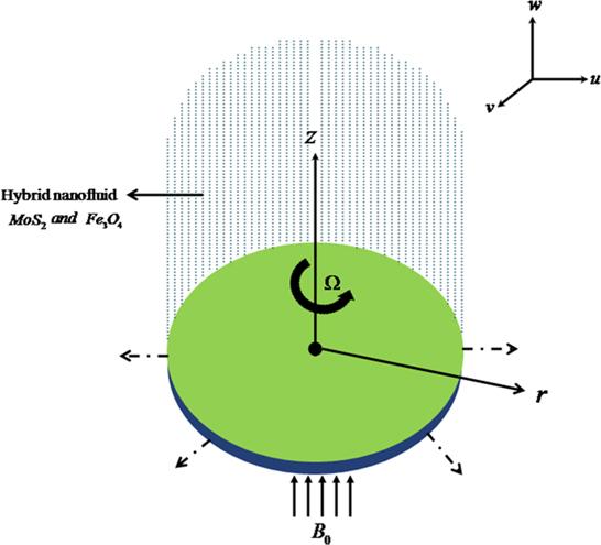
Figure 1. Flow configuration.
The modeled governing equations are as follows:
$\begin{eqnarray}\displaystyle \frac{\partial u}{\partial r}+\displaystyle \frac{\partial w}{\partial z}+\displaystyle \frac{u}{r}=0,\end{eqnarray}$
$\begin{eqnarray}\begin{array}{l}\left[u\displaystyle \frac{\partial u}{\partial r}+w\displaystyle \frac{\partial u}{\partial z}-\displaystyle \frac{{v}^{2}}{r}\right]=-\displaystyle \frac{1}{{\rho }_{{\rm{hnf}}}}\displaystyle \frac{\partial p}{\partial r}+\displaystyle \frac{{\mu }_{{\rm{hnf}}}}{{\rho }_{{\rm{hnf}}}}\\ \,\times \,\left[\displaystyle \frac{{\partial }^{2}u}{\partial {r}^{2}}+\displaystyle \frac{{\partial }^{2}u}{\partial {z}^{2}}+\displaystyle \frac{1}{r}\displaystyle \frac{\partial u}{\partial r}-\displaystyle \frac{u}{{r}^{2}}\right]-\displaystyle \frac{{\sigma }_{{\rm{hnf}}}}{{\rho }_{{\rm{hnf}}}}{B}_{0}^{2}u-\displaystyle \frac{{\mu }_{{\rm{hnf}}}}{K\,{\rho }_{{\rm{hnf}}}}u,\end{array}\end{eqnarray}$
$\begin{eqnarray}\begin{array}{l}\left[u\displaystyle \frac{\partial v}{\partial r}+w\displaystyle \frac{\partial v}{\partial z}+\displaystyle \frac{uv}{r}\right]=\displaystyle \frac{{\mu }_{{\rm{hnf}}}}{{\rho }_{{\rm{hnf}}}}\left[\displaystyle \frac{{\partial }^{2}v}{\partial {r}^{2}}+\displaystyle \frac{{\partial }^{2}v}{\partial {z}^{2}}+\displaystyle \frac{1}{r}\displaystyle \frac{\partial v}{\partial r}-\displaystyle \frac{v}{{r}^{2}}\right]\\ \,-\,\displaystyle \frac{{\sigma }_{{\rm{hnf}}}}{{\rho }_{{\rm{hnf}}}}{B}_{0}^{2}v-\displaystyle \frac{{\mu }_{{\rm{hnf}}}}{K\,{\rho }_{\mathrm{hnf}}}v,\end{array}\end{eqnarray}$
$\begin{eqnarray}\begin{array}{l}\left[u\displaystyle \frac{\partial w}{\partial r}+w\displaystyle \frac{\partial w}{\partial z}\right]=-\displaystyle \frac{1}{{\rho }_{{\rm{hnf}}}}\displaystyle \frac{\partial p}{\partial z}\\ \,+\,\displaystyle \frac{{\mu }_{{\rm{hnf}}}}{{\rho }_{{\rm{hnf}}}}\left[\displaystyle \frac{{\partial }^{2}w}{\partial {r}^{2}}+\displaystyle \frac{{\partial }^{2}w}{\partial {z}^{2}}+\displaystyle \frac{1}{r}\displaystyle \frac{\partial w}{\partial r}\right],\end{array}\end{eqnarray}$
$\begin{eqnarray}\begin{array}{l}\left[u\displaystyle \frac{\partial T}{\partial r}+w\displaystyle \frac{\partial T}{\partial z}\right]=\displaystyle \frac{{k}_{{\rm{hnf}}}}{{\left(\rho {C}_{{p}}\right)}_{{\rm{hnf}}}}\left[\displaystyle \frac{{\partial }^{2}T}{\partial {r}^{2}}+\displaystyle \frac{{\partial }^{2}T}{\partial {z}^{2}}+\displaystyle \frac{1}{r}\displaystyle \frac{\partial T}{\partial r}\right]\\ \,+\,\displaystyle \frac{2{\mu }_{{\rm{hnf}}}}{{\left(\rho {C}_{{p}}\right)}_{{\rm{hnf}}}}\left[{\left(\displaystyle \frac{\partial u}{\partial r}\right)}^{2}+\displaystyle \frac{{u}^{2}}{{r}^{2}}+{\left(\displaystyle \frac{\partial w}{\partial z}\right)}^{2}\right]+\displaystyle \frac{{\mu }_{{\rm{hnf}}}}{{\left(\rho {C}_{{p}}\right)}_{{\rm{hnf}}}}\\ \,\times \,\left[\begin{array}{c}{\left(\displaystyle \frac{\partial v}{\partial z}\right)}^{2}+{\left(\displaystyle \frac{\partial w}{\partial r}+\displaystyle \frac{\partial u}{\partial z}\right)}^{2}\\ +{\left[r\displaystyle \frac{\partial }{\partial z}\left(\displaystyle \frac{v}{r}\right)\right]}^{2}\end{array}\right]+\displaystyle \frac{{\sigma }_{{\rm{hnf}}}}{{\left(\rho {C}_{{p}}\right)}_{{\rm{hnf}}}}{B}_{0}^{2}\left({u}^{2}+{v}^{2}\right),\end{array}\end{eqnarray}$
$\begin{eqnarray}\begin{array}{l}\left[u\displaystyle \frac{\partial C}{\partial r}+w\displaystyle \frac{\partial C}{\partial z}\right]={D}_{{\rm{hnf}}}\left[\displaystyle \frac{{\partial }^{2}C}{\partial {r}^{2}}+\displaystyle \frac{{\partial }^{2}C}{\partial {z}^{2}}+\displaystyle \frac{1}{r}\displaystyle \frac{\partial C}{\partial r}\right]\\ \,-\,{k}_{{\rm{r}}}^{2}{\left(\displaystyle \frac{T}{{T}_{\infty }}\right)}^{n}{{\rm{e}}}^{-\tfrac{{E}_{{\rm{a}}}}{{k}^{* }T}}\,(C-{C}_{\infty }),\end{array}\end{eqnarray}$
with boundary conditions,
$\begin{eqnarray}\left.\begin{array}{l}z=0:u={a}_{1}r,v={\rm{\Omega }}r,w=0,T={T}_{w},C={C}_{w},\\ z\to \infty :u\to 0,v\to 0,w\to 0,T\to {T}_{\infty ,}C\to {C}_{\infty ,}P\to {P}_{\infty }.\end{array}\right\}\end{eqnarray}$
Here, $(u,v,w)$ are the velocity components T, ${T}_{{\rm{w}}},$ ${T}_{\infty }$, the temperature of the fluid, wall temperature and ambient temperature, respectively.
We consider the transformations:
$\begin{eqnarray}\begin{array}{l}u=r{\rm{\Omega }}f^{\prime} (\eta ),v=r{\rm{\Omega }}g(\eta ),\,w=-2\sqrt{{\nu }_{{\rm{f}}}{\rm{\Omega }}}f(\eta ),\\ \theta (\eta )=\displaystyle \frac{T-{T}_{\infty }}{{T}_{{\rm{w}}}-{T}_{\infty }},\chi (\eta )=\displaystyle \frac{C-{C}_{\infty }}{{C}_{{\rm{w}}}-{C}_{\infty }},\\ p={\rho }_{{\rm{f}}}{\rm{\Omega }}{\nu }_{{\rm{f}}}\left(P(\eta )+\displaystyle \frac{1}{2}\displaystyle \frac{{r}^{2}{\rm{\Omega }}}{{\nu }_{{\rm{f}}}}\varepsilon \right),\eta =\sqrt{\displaystyle \frac{{\rm{\Omega }}}{{\nu }_{{\rm{f}}}}}z.\end{array}\end{eqnarray}$
In view of equation (8), the continuity equation is satisfied exactly and equations (2)–(7) reduced as below:
$\begin{eqnarray}\begin{array}{l}f^{\prime\prime\prime} -\lambda f^{\prime} -{\left(1-{\varnothing }_{1}\right)}^{2.5}{\left(1-{\varnothing }_{2}\right)}^{2.5}\left[\left(1-{\varnothing }_{2}\right)\left[\begin{array}{c}\left(1-{\varnothing }_{1}\right)\\ +{\varnothing }_{1}\displaystyle \frac{{\rho }_{{\rm{s}}1}}{{\rho }_{{\rm{f}}}}\end{array}\right]\right.\\ \,+\,\left.{\varnothing }_{2}\displaystyle \frac{{\rho }_{{\rm{s}}2}}{{\rho }_{{\rm{f}}}}\right]\left[\begin{array}{c}{\left(f^{\prime} \right)}^{2}-2ff^{\prime\prime} \\ -{\left(g\right)}^{2}\end{array}\right]-\left[\displaystyle \frac{{\sigma }_{{\rm{hnf}}}}{{\sigma }_{{\rm{f}}}}Mf^{\prime} +\varepsilon \right]\\ \,\times \,{\left(1-{\varnothing }_{1}\right)}^{2.5}{\left(1-{\varnothing }_{2}\right)}^{2.5}=0,\end{array}\end{eqnarray}$
$\begin{eqnarray}\begin{array}{l}g^{\prime\prime} -\lambda g-{\left(1-{\varnothing }_{1}\right)}^{2.5}{\left(1-{\varnothing }_{2}\right)}^{2.5}\left[\left(1-{\varnothing }_{2}\right)\left[\begin{array}{c}\left(1-{\varnothing }_{1}\right)\\ +{\varnothing }_{1}\displaystyle \frac{{\rho }_{{\rm{s}}1}}{{\rho }_{{\rm{f}}}}\end{array}\right]\right.\\ \,+\,\left.{\varnothing }_{2}\displaystyle \frac{{\rho }_{{\rm{s}}2}}{{\rho }_{{\rm{f}}}}\right]\left[2f^{\prime} g-2fg^{\prime} \right]-\left[\displaystyle \frac{{\sigma }_{{\rm{hnf}}}}{{\sigma }_{{\rm{f}}}}Mg\right]\\ \,\times \,{\left(1-{\varnothing }_{1}\right)}^{2.5}{\left(1-{\varnothing }_{2}\right)}^{2.5}=0,\end{array}\end{eqnarray}$
$\begin{eqnarray}\begin{array}{l}f^{\prime\prime} +{\left(1-{\varnothing }_{1}\right)}^{2.5}{\left(1-{\varnothing }_{2}\right)}^{2.5}\left[\begin{array}{c}\left(1-{\varnothing }_{2}\right)\left[\begin{array}{c}\left(1-{\varnothing }_{1}\right)\\ +{\varnothing }_{1}\displaystyle \frac{{\rho }_{{\rm{s}}1}}{{\rho }_{{\rm{f}}}}\end{array}\right]\\ +{\varnothing }_{2}\displaystyle \frac{{\rho }_{{\rm{s}}2}}{{\rho }_{{\rm{f}}}}\end{array}\right]2ff^{\prime} \\ \,+\,\displaystyle \frac{1}{2}P^{\prime} {\left(1-{\varnothing }_{1}\right)}^{2.5}{\left(1-{\varnothing }_{2}\right)}^{2.5}=0,\end{array}\end{eqnarray}$
$\begin{eqnarray}\begin{array}{l}\displaystyle \frac{{k}_{{\rm{hnf}}}}{{k}_{{\rm{f}}}}{\theta }^{{\prime\prime} }+2{\Pr }\left[\left(1-{\varnothing }_{2}\right)\left[\begin{array}{c}\left(1-{\varnothing }_{1}\right)\\ +{\varnothing }_{1}\displaystyle \frac{{\left(\rho C{\rm{p}}\right)}_{{\rm{s}}1}}{{\left(\rho C{\rm{p}}\right)}_{{\rm{f}}}}\end{array}\right]+{\varnothing }_{2}\displaystyle \frac{{\left(\rho C{\rm{p}}\right)}_{{\rm{s}}2}}{{\left(\rho C{\rm{p}}\right)}_{{\rm{f}}}}\right]\theta ^{\prime} f\\ \,-\,\displaystyle \frac{12Ec{\Pr }}{\mathrm{Re}}{\left(f^{\prime} \right)}^{2}+{\Pr }Ec\left(\begin{array}{c}{\left(f^{\prime\prime} \right)}^{2}\\ +{\left(g^{\prime} \right)}^{2}\end{array}\right)\\ \,+\,\displaystyle \frac{{\sigma }_{{\rm{hnf}}}}{{\sigma }_{{\rm{f}}}}{\Pr }MEc\left[{\left(f^{\prime} \right)}^{2}+{\left(g\right)}^{2}\right]=0,\end{array}\,\end{eqnarray}$
$\begin{eqnarray}\begin{array}{l}{\left(1-{\varnothing }_{1}\right)}^{2.5}{\left(1-{\varnothing }_{2}\right)}^{2.5}\chi ^{\prime\prime} +2Scf\chi ^{\prime} -Sc\sigma {(1+\delta \theta )}^{n}\\ \,\times \,\exp \left(-\displaystyle \frac{E}{(1+\delta \theta )}\right)\chi =0.\end{array}\,\end{eqnarray}$
Similarly, the transformed boundary conditions are:
$\begin{eqnarray}\left.\begin{array}{l}f^{\prime} (0)=A,g(0)=1,f(0)=0,\theta (0)=1,\chi (0)=1,\\ f^{\prime} (\infty )\to 0,g(\infty )\to 0,f(\infty )\to 0,\theta (\infty )\to 0,\chi (\infty )\to 0.\end{array}\right\}\end{eqnarray}$
where
$\begin{eqnarray*}\begin{array}{l}\lambda =\displaystyle \frac{{\nu }_{{\rm{f}}}}{K{\rm{\Omega }}},Sc=\displaystyle \frac{{\nu }_{{\rm{f}}}}{{D}_{{\rm{f}}}},M=\displaystyle \frac{{\sigma }_{{\rm{f}}}{B}_{0}^{2}}{{\rho }_{{\rm{f}}}{\rm{\Omega }}},Ec=\displaystyle \frac{{r}^{2}{{\rm{\Omega }}}^{2}}{{C}_{{p}}\left({T}_{{\rm{w}}}-{T}_{\infty }\right)},\\ {\Pr }=\displaystyle \frac{{\nu }_{{\rm{f}}}{(\rho {C}_{{p}})}_{{\rm{f}}}}{{k}_{{\rm{f}}}},\sigma =\displaystyle \frac{{k}_{r}^{2}}{{\rm{\Omega }}},E=\displaystyle \frac{{E}_{{\rm{a}}}}{{k}^{* }{T}_{\infty }},\delta =\displaystyle \frac{{T}_{{\rm{w}}}-{T}_{\infty }}{{T}_{\infty }}\\ {\rm{and}}\,{Re}\,=\,\displaystyle \frac{{r}^{2}{\rm{\Omega }}}{{\nu }_{{\rm{f}}}}.\end{array}\end{eqnarray*}$
Here, $\sigma $ -reaction rate, $E$ -activation energy, $\delta \,$-temperature difference and $\lambda ,$ $Sc,M,Ec,\Pr ,\mathrm{Re},A$ are the porosity parameter, Schmidt number, Hartmann number, Eckert number, Prandtl number, local Reynolds number and stretching parameter, respectively.
Equation (9) is differentiated with respect to $\eta $ as follows:
$\begin{eqnarray}\begin{array}{l}{f}^{iv}-\lambda f^{\prime\prime} +{\left(1-{\varnothing }_{1}\right)}^{2.5}{\left(1-{\varnothing }_{2}\right)}^{2.5}\left[\left(1-{\varnothing }_{2}\right)\left[\begin{array}{c}\left(1-{\varnothing }_{1}\right)\\ +{\varnothing }_{1}\displaystyle \frac{{\rho }_{{\rm{s}}1}}{{\rho }_{{\rm{f}}}}\end{array}\right]\right.\\ \,+\,\left.{\varnothing }_{2}\displaystyle \frac{{\rho }_{{\rm{s}}2}}{{\rho }_{{\rm{f}}}}\right]\left[2ff^{\prime\prime\prime} +2gg^{\prime} \right]-\left[\displaystyle \frac{{\sigma }_{{\rm{hnf}}}}{{\sigma }_{{\rm{f}}}}Mf^{\prime\prime} \right]{\left(1-{\varnothing }_{1}\right)}^{2.5}\\ \,\times \,{\left(1-{\varnothing }_{2}\right)}^{2.5}=0,\end{array}\end{eqnarray}$
where, (${\rho }_{{\rm{hnf}}},$ ${\mu }_{{\rm{hnf}}},$ ${k}_{{\rm{hnf}}}$ and ${\left(\rho {C}_{{p}}\right)}_{{\rm{hnf}}}$) are given below:
$\begin{eqnarray*}{D}_{{\rm{hnf}}}={(1-{\varnothing }_{1})}^{2.5}{(1-{\varnothing }_{2})}^{2.5}{D}_{{\rm{f}}},\end{eqnarray*}$
$\begin{eqnarray*}{\mu }_{{\rm{hnf}}}=\displaystyle \frac{{\mu }_{{\rm{f}}}}{{\left(1-{\varnothing }_{1}\right)}^{2.5}{\left(1-{\varnothing }_{2}\right)}^{2.5}},\end{eqnarray*}$
$\begin{eqnarray*}\displaystyle \frac{{\rho }_{{\rm{hnf}}}}{{\rho }_{{\rm{f}}}}=\left(1-{\varnothing }_{2}\right)\left[\left(1-{\varnothing }_{1}\right)+{\varnothing }_{1}\displaystyle \frac{{\rho }_{{\rm{s}}1}}{{\rho }_{{\rm{f}}}}\right]+{\varnothing }_{2}\displaystyle \frac{{\rho }_{{\rm{s}}2}}{{\rho }_{{\rm{f}}}},\end{eqnarray*}$
$\begin{eqnarray*}\begin{array}{l}\displaystyle \frac{{\left(\rho {C}_{{p}}\right)}_{{\rm{hnf}}}}{{\left(\rho {C}_{{p}}\right)}_{{\rm{f}}}}=\left(1-{\varnothing }_{2}\right)\left[\left(1-{\varnothing }_{1}\right)+{\varnothing }_{1}\left(\displaystyle \frac{{\left(\rho {C}_{{p}}\right)}_{{\rm{s}}1}}{{\left(\rho {C}_{{p}}\right)}_{{\rm{f}}}}\right)\right]\\ \,\,\,\,\,+\,{\varnothing }_{2}\displaystyle \frac{{\left(\rho {C}_{{p}}\right)}_{{\rm{s}}2}}{{\left(\rho {C}_{{p}}\right)}_{{\rm{f}}}},\end{array}\end{eqnarray*}$
$\begin{eqnarray*}\begin{array}{l}\displaystyle \frac{{k}_{{\rm{hnf}}}}{{k}_{{\rm{bf}}}}=\displaystyle \frac{{k}_{{{\rm{s}}}_{2}}+2{k}_{{\rm{bf}}}-2{\varnothing }_{2}\left({k}_{{\rm{bf}}}-{k}_{{{\rm{s}}}_{2}}\right)}{{k}_{{{\rm{s}}}_{2}}+2{k}_{{\rm{bf}}}+{\varnothing }_{2}\left({k}_{{\rm{bf}}}-{k}_{{{\rm{s}}}_{2}}\right)},\\ \displaystyle \frac{{k}_{{\rm{bf}}}}{{k}_{{\rm{f}}}}=\displaystyle \frac{{k}_{{{\rm{s}}}_{1}}+2{k}_{{\rm{f}}}-2{\varnothing }_{1}\left({k}_{{\rm{f}}}-{k}_{{{\rm{s}}}_{1}}\right)}{{k}_{{{\rm{s}}}_{1}}+2{k}_{{\rm{f}}}+{\varnothing }_{1}\left({k}_{{\rm{f}}}-{k}_{{{\rm{s}}}_{1}}\right)},\end{array}\end{eqnarray*}$
$\begin{eqnarray*}\begin{array}{l}{\sigma }_{{\rm{hnf}}}=\displaystyle \frac{{\sigma }_{{s}_{2}}+2{\sigma }_{{\rm{bf}}}-2{\varnothing }_{2}\left({\sigma }_{{\rm{bf}}}-{\sigma }_{{s}_{2}}\right)}{{\sigma }_{{s}_{2}}+2{\sigma }_{{\rm{bf}}}+{\varnothing }_{2}\left({\sigma }_{{\rm{bf}}}-{\sigma }_{{s}_{2}}\right)},\\ \displaystyle \frac{{\sigma }_{{\rm{bf}}}}{{\sigma }_{{\rm{f}}}}=\displaystyle \frac{{\sigma }_{{{\rm{s}}}_{1}}+2{\sigma }_{{\rm{f}}}-2{\varnothing }_{1}\left({\sigma }_{{\rm{f}}}-{\sigma }_{{{\rm{s}}}_{2}}\right)}{{\sigma }_{{{\rm{s}}}_{1}}+2{\sigma }_{{\rm{f}}}+{\varnothing }_{1}\left({\sigma }_{{\rm{f}}}-{\sigma }_{{{\rm{s}}}_{2}}\right)},\end{array}\end{eqnarray*}$
where ${\rho }_{{\rm{f}}},$ ${\rho }_{{\rm{s}}1},$ ${\rho }_{{\rm{s}}2},$ ${({C}_{{p}})}_{{\rm{f}}},$ ${({C}_{{p}})}_{{\rm{s}}1},$ ${({C}_{{p}})}_{{\rm{s}}2}$ represent density of fluid, solid nanoparticles of ${{\rm{MoS}}}_{2},$ solid nanoparticles of ${{\rm{Fe}}}_{3}{{\rm{O}}}_{4},$ specific heat of hybrid nanofluid, base fluid, solid nanoparticles of ${{\rm{MoS}}}_{2}$ and solid nanoparticles of ${{\rm{Fe}}}_{3}{{\rm{O}}}_{4}$, respectively. ${k}_{{\rm{f}}},$ ${k}_{{\rm{s}}1},$ ${k}_{{\rm{s}}2}$ are the thermal conductivity of base fluid, solid nanoparticles of ${{\rm{MoS}}}_{2}$ and solid nanoparticles of ${{\rm{Fe}}}_{3}{{\rm{O}}}_{4}.$ ${\sigma }_{{\rm{f}}},$ ${\sigma }_{{\rm{f}}},$ ${\sigma }_{{\rm{s}}1},$ ${\sigma }_{{\rm{s}}2},$ ${\sigma }_{{\rm{bf}}}$ are the electrical conductivity of a fluid, solid particles and base fluid.
The $Sh,$ $Nu$ and ${C}_{{\rm{f}}}$ are given as:
$\begin{eqnarray*}\begin{array}{l}Sh=\displaystyle \frac{r{j}_{{\rm{w}}}}{{D}_{{\rm{hnf}}}\left({C}_{{\rm{w}}}-{C}_{\infty ,}\right)},Nu=\displaystyle \frac{r{q}_{{\rm{w}}}}{{k}_{{\rm{f}}}\left({T}_{{\rm{w}}}-{T}_{\infty }\right)},\\ {C}_{{\rm{fx}}}=\displaystyle \frac{\sqrt{{{\tau }_{{\rm{wt}}}}^{2}+{{\tau }_{{\rm{w}}\phi }}^{2}}}{{\rho }_{{\rm{f}}}{\left({\rm{\Omega }}r\right)}^{2}}.\end{array}\end{eqnarray*}$
Here, ${\tau }_{{\rm{wt}}},$ ${\tau }_{{\rm{w}}\phi },$ ${{\rm{q}}}_{{\rm{w}}}$ and ${j}_{{\rm{w}}}$ are as follows:
$\begin{eqnarray*}\begin{array}{l}{\tau }_{{\rm{wt}}}={\left[{\mu }_{{\rm{hnf}}}\left(\displaystyle \frac{\partial u}{\partial z}+\displaystyle \frac{\partial w}{\partial \phi }\right)\right]}_{z=0},\\ {\tau }_{{\rm{w}}\phi }={\left[{\mu }_{{\rm{hnf}}}\left(\displaystyle \frac{\partial v}{\partial z}+\displaystyle \frac{1}{r}\displaystyle \frac{\partial w}{\partial \phi }\right)\right]}_{z=0},\\ {q}_{{\rm{w}}}=-{k}_{{\rm{hnf}}}{\left(\displaystyle \frac{\partial T}{\partial z}\right)}_{z=0}\,{\rm{and}}\,{j}_{{\rm{w}}}=-{D}_{{\rm{hnf}}}{\left(\displaystyle \frac{\partial C}{\partial z}\right)}_{z=0}.\end{array}\end{eqnarray*}$
The non-dimensional form of ${{Re}}^{-1/2}Sh,$ ${{Re}}^{-1/2}Nu$ and ${{Re}}^{1/2}{C}_{{\rm{fx}}}$ are:
$\begin{eqnarray*}\begin{array}{l}{{Re}}^{-\tfrac{1}{2}}Sh=-\chi ^{\prime} (0),{{Re}}^{-\tfrac{1}{2}}Nu=-\displaystyle \frac{{k}_{{\rm{hnf}}}}{{k}_{{\rm{f}}}}\theta ^{\prime} \left(0\right),\\ {\rm{and}}\,{{Re}}^{\tfrac{1}{2}}{C}_{{\rm{fx}}}=\displaystyle \frac{\sqrt{{\left(f^{\prime\prime} (0)\right)}^{2}+{\left(g^{\prime} (0)\right)}^{2}}}{{\left(1-{\phi }_{1}\right)}^{2.5}{\left(1-{\phi }_{2}\right)}^{2.5}},\end{array}\end{eqnarray*}$
where ${Re}\,=\,\tfrac{{\rm{\Omega }}{r}^{2}}{{\nu }_{{\rm{f}}}}$ is the local Reynolds number.

3. Result and discussion

This section covers the outcomes of the MHD flow over a rotating disk with suspension of different nanoparticles. Two types of oxides, namely molybdenum disulfide and ferro sulfate, are suspended in base fluid water. The powerful numerical mechanism RKF fourth-fifth order along with a shooting technique is used to deal the non-dimensional governing equations of the present problem. Table 1 presents the thermo-physical properties of each base fluid and the nanoparticles. In order to provide insight, the effects of various governing parameters on the $f^{\prime} (\eta ),$ $g\left(\eta \right),$ $\theta \left(\eta \right)$ and $\chi \left(\eta \right)$ are discussed graphically.
Table 1. Thermo-physical properties of nanoparticles.
Physical properties Base fluid ${{\rm{H}}}_{2}{\rm{O}}$ Nanoparticles ${{\rm{MoS}}}_{2}$ Nanoparticles ${{\rm{Fe}}}_{3}{{\rm{O}}}_{4}$
Density $\rho ({\rm{kg}}\,{{\rm{m}}}^{-3})$ 997.1 5060 5180
Specific heat ${c}_{{p}}({\rm{J}}/{\rm{kgK}})$ 4179 397 670
Thermal conductivity $k({\rm{W}}\,{{\rm{mK}}}^{-1})$ 0.613 904.4 9.7
Electrical conductivity $\sigma {\left({\rm{\Omega }}{\rm{m}}\right)}^{-1}$ $5.5\times {10}^{-6}$ 2090 25 000
Figures 24 show the domination of $M$ over $f^{\prime} (\eta ),$ $g\left(\eta \right),$ and $\theta \left(\eta \right)$ for the cases of hybrid nanoparticles and nanoparticles. Here, an escalating integrity of $M$ decays the $f^{\prime} (\eta ),$ and $g\left(\eta \right)$ (see figures 2 and 3). Likewise, the thickness of the corresponding layer reduces for enhanced values of $M.$ In addition, the velocity of the fluid is lower in nanofluid when treated with hybrid nanofluid. Substantially larger values of $M$ increased the Lorenz force. Consequently, the accelerated Lorentz force generates extra drag to the ambulation of the fluid flow and nanoparticles. From figure 4 it can be seen that $\theta \left(\eta \right)$ results in larger integrities of $M.$ Furthermore, the corresponding thermal field increases for larger $M.$ The impact of $\lambda $ on $f^{\prime} (\eta ),$ and $g\left(\eta \right)$ is shown in figures 5, 6. Here, it is contemplated that the escalating values of $\lambda $ decrease both the profiles $f^{\prime} (\eta ),$ and $g\left(\eta \right)$ of both the nanoparticle and hybrid nanoparticle case. Besides the interrelated thickness of the layer scales back for larger $\lambda .$ In addition, the velocity of the fluid is lower in nanoparticles when treated with hybrid nanoparticles.
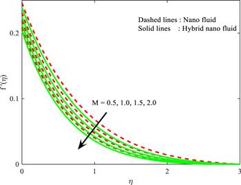
Figure 2. Influence of $M$ on $f^{\prime} \left(\eta \right).$
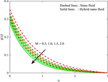
Figure 3. Influence of $M$ on $g\left(\eta \right).$
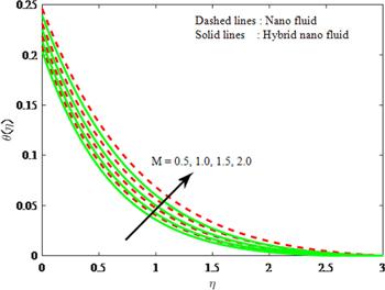
Figure 4. Influence of $M$ on $\theta \left(\eta \right).$
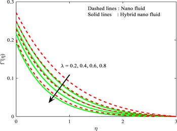
Figure 5. Influence of $\lambda $ on $f^{\prime} \left(\eta \right).$
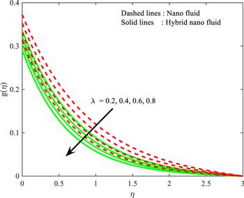
Figure 6. Influence of $\lambda $ on $g\left(\eta \right).$
The influence of ${\varnothing }_{1}$ on $f^{\prime} (\eta ),$ and $\theta \left(\eta \right)$ profiles for both ${{\rm{MoS}}}_{2}-{{\rm{H}}}_{2}{\rm{O}}$ and ${{\rm{Fe}}}_{3}{{\rm{O}}}_{4}-{{\rm{H}}}_{2}{\rm{O}}$ nanoparticle cases are depicted in figures 7, 8. Here, it is noted enlarged values of volume fraction declines the velocity profile, but enhances the thermal profile. Furthermore, the compactness of the corresponding layers also provides for growing values of $K.$ Furthermore, the enhancement of fluid flow is higher in nanoparticles than that of hybrid nanoparticles. Figures 9, 10 reproduce $f^{\prime} (\eta ),$ and $\theta \left(\eta \right)$ of both the hybrid nanoparticle and nanoparticle case for different values of ${\varnothing }_{2}.$ One may observe from these figure that the velocity profile is declined and thermal profile is enhanced for increased integrates of volume fraction ${\varnothing }_{2}.\,\,$The compactness of momentum of both hybrid nanoparticle and nanoparticle cases declines for increasing values of ${\varnothing }_{2}$ parameter, but the opposite trend can be seen for thermal profile.
Figure 7. Influence of ${\varnothing }_{1}$ on $f^{\prime} \left(\eta \right).$
Figure 8. Influence of ${\varnothing }_{1}\,$on $\theta \left(\eta \right).$
Figure 9. Influence of ${\varnothing }_{2}$ on $f^{\prime} \left(\eta \right).$
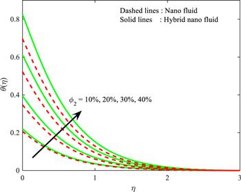
Figure 10. Influence of ${\varnothing }_{2}$ on $\theta \left(\eta \right).$
The influence of Eckert number on the thermal field of the nanofluid and hybrid nanofluid is displayed in figure 11. The increasing Eckert number increases the thermal field. In the case of a large magnetic force system, the major disruption of the temperature field induced by each member is an interesting result. These physical phenomena are attributable to the cumulative effect of heat energy stored in the nanofluid and hybrid nanofluid due to fractional heating. The variation in thermal field of the nanofluid and hybrid nanofluid versus Prandtl number ${\Pr }$ is shown in figure 12. The graph shows that the thermal field and thermal layer thickness decline whenever the ${\Pr }$ values are boosted. This is really caused by the fact that with the greater Prandtl number, fluids will have a comparatively low conductivity, which mostly diminishes the heat transfer and thickness of the thermal fluid flow and therefore the temperature of the fluid reduces. The effect of $\Pr $ on Newtonian fluids is close to what we are seeing in nanofluid. These characteristics are thus already retained by nanofluids.
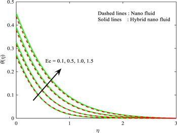
Figure 11. Influence of $Ec$ on $\theta \left(\eta \right).$
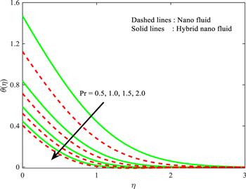
Figure 12. Influence of ${\Pr }$ on $\theta \left(\eta \right).$
Figure 13 shows the denouement of the $Sc$ parameter on the $\chi (\eta )$ profile for both the nanoparticle and hybrid nanoparticle case. Here, it is essential to mention that the extreme values of $Sc$ scale back the fluid concentration. Furthermore, the solutal layer of both the nanoparticle and hybrid nanoparticle case reduces for higher values of $Sc.$ The influence of $\sigma $ on the solutal field of the nanofluid and hybrid nanofluid is shown in figure 14. One may observe that the solutal field is scaled back for increment values of $\sigma .$ The compactness of the solutal layer of both the hybrid nanoparticle and nanoparticle case reduces for increasing values of the material parameter. In addition, the concentration of the fluid is much faster in the nanoparticle case when compared with the hybrid nanoparticle case. The $\sigma $ and $E$ on $\chi (\eta )$ for both the hybrid nanoparticle and nanoparticle case are depicted in figures 15, 16. Here, it is observed that an increasing value of $E$ scales back the concentration of the fluid flow in both nanoparticle cases.
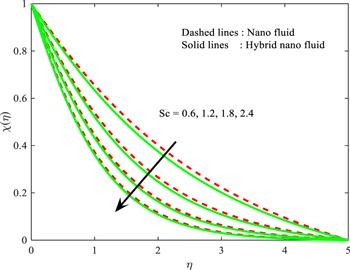
Figure 13. Influence of $Sc$ on $\chi \left(\eta \right).$
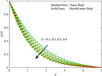
Figure 14. Influence of $\delta $ on $\chi \left(\eta \right).$
Figure 15. Influence of $\sigma $ on $\chi \left(\eta \right).$
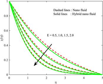
Figure 16. Influence of $E$ on $\chi \left(\eta \right).$
The impact of $\lambda $ and ${\varnothing }_{1}$ on ${{Re}}^{1/2}{C}_{{\rm{fx}}}$ is delineated in figure 17. Here, it is contemplated that the escalating values of $\lambda $ and ${\varnothing }_{1}$ scale back the friction factor for both the hybrid nanoparticle and nanoparticle case. Besides, there is an interrelated thickness of the layer downturn for larger $\lambda $ and ${\varnothing }_{1}.$ Furthermore, the reduction of the friction factor is less in hybrid nanoparticles when compared to nanoparticles. Figure 18 represents the encounter of $Ec$ and ${\Pr }$ on ${{Re}}^{-1/2}Nu$ for both the hybrid nanoparticle and nanoparticle case. One may observe that boosted values of $\Pr $ reduce the temperature of the fluid for both the hybrid nanoparticle and nanoparticle case. Hence, ${{Re}}^{-1/2}Nu$ is scaled back, while the opposite trend is observed for higher values of $Ec.$ Figure 19 reproduces the ${{Re}}^{-1/2}Sh$ for varying $Sc$ and $\delta $ for both the hybrid nanoparticle and nanoparticle case. Here, it is essential to mention that larger values of $Ec$ enhance the ${{Re}}^{-1/2}Sh$ in both the hybrid nanoparticle and nanoparticle case.
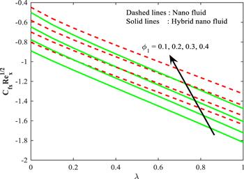
Figure 17. Influence of $\lambda $ versus ${\varnothing }_{1}$ on ${{Re}}^{\tfrac{1}{2}}{C}_{{\rm{fx}}}.$
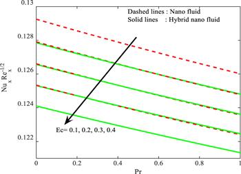
Figure 18. Influence of $Ec$ and ${\Pr }$ on ${{Re}}^{-1/2}Nu.$
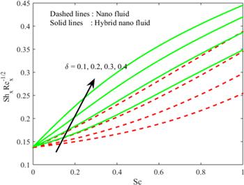
Figure 19. Influence of $\delta $ and $Sc$ on ${{Re}}^{-1/2}Sh.$
The effects of diversified governing flow parameters on the friction coefficients ${{Re}}^{1/2}{C}_{{\rm{fx}}},$ ${{Re}}^{-1/2}Nu$ and ${{Re}}^{-1/2}Sh$ are listed in tables 24. From table 2, it can be seen that the fiction coefficient is enhanced by increasing $M$ and $\lambda ,$ but a reverse trend is observed for both ${\varnothing }_{1}\,\,$and ${\varnothing }_{2}.$ Furthermore, from table 2 it is noted that the value of the heat transfer rate scale back can be established by accumulating values of $\Pr ,{\varnothing }_{1}$ and ${\varnothing }_{2}.$ While, a reverse trend is observed for booster values of both $M$ and $Ec.$ From table 4 it can be seen that the rate of mass transfer declined for increasing values of $Sc\,\,$and $\sigma .$ Table 5 gives the comparison of statistical values of the current problem with published results and it shows good agreement.
Table 2. Numerical values of ${{Re}}^{\tfrac{1}{2}}{C}_{{\rm{fx}}}$ for different physical parameter values.
${{Re}}^{\tfrac{1}{2}}{C}_{{\rm{fx}}}$
$M$ $\lambda $ ${\varnothing }_{1}$ ${\varnothing }_{2}$ Nanofluid Hybrid nanofluid
0.5 −1.127 498 −1.106 825
1.0 −1.177 467 −1.153 211
1.5 −1.192 089 −1.192 160
0.1 0.977 902 −1.094 206
0.2 −−1.084 503 −1.145 167
0.3 −1.144 617 −1.199 912
0.1 −0.137 800 −0.184 883
0.2 −0.122 279 −0.164 147
0.3 −0.106 240 −0.142 617
0.1 −0.144 872 −0.157 821
0.2 −0.125 478 −0.148 756
0.3 −0.104 887 −0.954 71
Table 3. Numerical values of ${{Re}}^{-1/2}Nu$ for different physical parameter values for both the hybrid and nanofluid case.
${{Re}}^{-1/2}Nu$
${\Pr }$ $Ec$ $M$ ${\varnothing }_{1}$ ${\varnothing }_{2}$ Nanofluid Hybrid nanofluid
0.1 0.147 526 0.166 076
0.3 0.171 266 0.166 270
0.5 0.201 602 0.201 61
0.1 0.262 315 0.171 266
0.3 0.238 968 0.166 031
0.5 0.218 061 0.161 655
0.1 0.184 255 0.179 411
0.2 0.187 977 0.180 097
0.3 0.192 973 0.183 820
0.1 2.452 295 2.457 524
0.2 2.349 007 2.359 885
0.3 2.241 073 2.258 100
0.1 2.632 48 2.527 524
0.2 2.415 200 2.429 885
0.3 2.351 073 2.338 100
Table 4. Numerical values of ${{Re}}^{-1/2}Sh$ for different physical parameter values for both the hybrid and nanofluid case.
${{Re}}^{-1/2}Sh$
$Sc$ $\sigma $ $\delta $ $E$ Nano fluid Hybrid nanofluid
0.1 0.594 632 0.682 126
0.2 0.622 126 0.757 120
0.3 0.737 120 0.833 300
0.1 0.228 075 0.239 495
0.15 0.259 495 0.300 374
0.2 0.278 075 0.319 495
0.1 0.378 485 0.390 374
0.2 0.350 374 0.360 687
0.3 0.378 485 0.390 374
0.01 0.250 454 0.270 687
0.1 0.287 421 0.288 215
0.2 0.304 821 0.314 562
Table 5. Comparison of of statistical values with Miklavcic and Wang [36] in the absence of $M,$ $\varepsilon ,$ $\lambda $ Pressure gradient, nanoparticles, energy and mass effects.
Miklavcic and Wang [36] Present results
A $\eta $ $f^{\prime\prime} (0)$ $g^{\prime} (0)$ $f^{\prime\prime} (0)$ $g^{\prime} (0)$
0.0 0.0 0.510 232 −0.615 922 0.509 680 −0.605 830

4. Conclusion

A hybrid nanoparticle performance of Arrhenius activation energy over a rotating disk by considering MHD is examined numerically. A powerful numerical mechanism RKF fourth and fifth order by adopting a shooting approach is used to deal with the non-dimensional governing equations of the present problem. The outcome of the velocity, concentration and temperature profile of both nanoparticle cases for distinct values of non-dimensional parameter are presented graphically and analyzed. Based on these graphs and tables we conclude that:

enhanced values of $\lambda $ decrease the velocity profile for both cases

enhancement of heat transfer is greater in hybrid nanoparticles when compared to nanoparticles for different values of $M$

$f^{\prime} (\eta )$ and $g(\eta )$ is decreased for enhancing values of both ${\varnothing }_{1}\,\,$and ${\varnothing }_{2}$

larger $\sigma $ and $Sc$ reduces the solutal boundary layer

larger-scale $M$ and $\lambda $ slows down the fluid velocity of both nanoparticle cases

thermal field enhances for increasing values of both ${\varnothing }_{1}\,\,$and ${\varnothing }_{2}.$

Future work may add further value to the present topic by the investigation of hybrid nanofluid flow through new physical mechanisms, relevant influencing factors and a combination of different nanoparticles suspended in diverse carrier liquids.

The authors gratefully acknowledge the financial support from Dr D S Kothari Post-Doctoral Fellowship Scheme, University Grants Commission, New Delhi.

1
Menzinger M Wolfgang R 1969 The meaning and use of the Arrhenius activation energy AngewandteChemie International Edition in English 8 438 444

DOI

2
Jensen F 1985 Activation energies and the Arrhenius equation Qual. Reliab. Eng. Int. 1 13 17

DOI

3
Hayat T Khan S A Khan M I Alsaedi A 2018 Impact of activation energy in nonlinear mixed convective chemically reactive flow of third grade nanomaterial by a rotating disk Int. J. Chem. Reactor Eng. 17 20180170

DOI

4
Khan N S Kumam P Thounthong P 2020 Second law analysis with effects of Arrhenius activation energy and binary chemical reaction on nanofluid flow Sci. Rep. 10 1226

DOI

5
Salahuddin T Arshad M Siddique N Alqahtani A S Malik M Y 2020 Thermophysical properties and internal energy change in Casson fluid flow along with activation energy Ain Shams Engineering Journal 11 1355 1365

DOI

6
Kumar K G Baslem A Prasannakumara B C Majdoubi J Gorji M R Nadeem S 2020 Significance of Arrhenius activation energy in flow and heat transfer of tangent hyperbolic fluid with zero mass flux condition Microsystem and technology 26 2517 2526

DOI

7
Khan M I Nasir T Hayat T Khan N B Alsaedi A 2020 Binary chemical reaction with activation energy in rotating flow subject to nonlinear heat flux and heat source/sink Journal of Computational Design and Engineering 7 279 286

DOI

8
Asma M Othman W A Muhammad T Mallawi F Wong B R 2019 Numerical study for magnetohydrodynamic flow of nanofluid due to a rotating disk with binary chemical reaction and Arrhenius activation energy Symmetry 11 1282

DOI

9
Ramzan M Bilal M Chung J D 2017 Radiative flow of Powell-Eyring magneto-nanofluid over a stretching cylinder with chemical reaction and double stratification near a stagnation point PLoS One 12 1 19

DOI

10
Zeeshan A Shehzad N Ellahi R 2018 Analysis of activation energy in Couette-Poiseuille flow of nanofluid in the presence of chemical reaction and convective boundary conditions Results in Physics 8 502 512

DOI

11
El-Hakiem M A Ramzan M Chung J D 2016 A numerical study of magnetohydrodynamic stagnation point flow of nanofluid with Newtonian heating Journal of Computational and Theoretical NanoScience 13 8419 8426

DOI

12
Lu D C Ramzan M Huda N U 2018 Nonlinear radiation effect on MHD Carreau nanofluid flow over a radially stretching surface with zero mass flux at the surface Sci. Rep. 8 1 16

DOI

13
Khan M Humara S Hasim 2018 Heat generation/absorption and thermal radiation impacts on three-dimensional flow of Carreau fluid with convective heat transfer J. Mol. Liq. 18 474 480

DOI

14
Reddy M G Sandeep N 2018 Heat and mass transfer in radiative MHD Carreau fluid with cross diffusion Ain Shams Eng. J. 9 1189 1204

DOI

15
Von Karman T 1921 Uber laminate und turbulent reibung Z Angew Math Mech. 1 233 252

DOI

16
Turkyilmazoglu M 2012 MHD fluid flow and heat transfer due to a stretching rotating disk Int. J. Therm. Sci. 51 195 201

DOI

17
Turkyilmazoglu M 2014 Nanofluid flow and heat transfer due to a rotating disk Comput. Fluids 94 139 146

DOI

18
Hayat T Javed M Imtiaz M Alsaedi A 2017 Convective flow of Jeffrey nanofluid due to two stretchable rotating disks J. Mol. Liq. 240 291 302

DOI

19
Yin C Zheng L Zhang C Zhang X 2017 Flow and heat transfer of nanofluids over a rotating disk with uniform stretching rate in the radial direction Propulsion and Power Research 6 25 30

DOI

20
Hayat T Khalid H Waqas M Alsaedi A 2018 Numerical simulation for radiative flow of nano liquid by rotating disk with carbon nanotubes and partial slip Comput. Meth. Appl. Mech. Eng. 341 397 408

DOI

21
Rehman K U Malik M Y Khan W A Khan I Alharbi S O 2019 Numerical solution of non-Newtonian fluid flow due to rotatory rigid disk Symmetry 11 699

DOI

22
Rafiq T Mustafa M 2019 Computational analysis of unsteady swirling flow around a decelerating rotating porous disk in nanofluid Arab. J. Sci. Eng. 45 1143 1154

DOI

23
Turkyilmazoglu M 2020 Suspension of dust particles over a stretchable rotating disk and two-phase heat transfer Int. J. Multiphase Flow 127 103260

DOI

24
Assaddiq A Khan S Bilal M Gul T Mukhtar S Shah Z Bonyah E 2020 Heat and mass transfer together with hybrid nanofluid flow over a rotating disk AIP Adv. 10 055317

DOI

25
Ramesh G K Kumara B C P Gireesha B J Gorla R S R 2015 MHD stagnation point flow of nanofluid towards a stretching surface with variable thickness and thermal radiation J Nanofluids 4 247 253

DOI

26
Sheikholeslami M Shehzad S A Kumar R 2018 Natural convection of Fe3O4-ethylene glycol nanouid under the impact of electric field in a porous enclosure Commun. Theor. Phys. 69 667

DOI

27
Kumar R Kumar R Koundal R Shehzad S A Sheikholeslami M 2019 Cubic auto-catalysis reactions in three-dimensional nanofluid flow considering viscous and Joule dissipations under thermal jump Commun. Theor. Phys. 71 779

DOI

28
Sharma A Tripathi D Sharma R K Tiwari A K 2019 Analysis of double diffusive convection in electroosmosis regulated peristaltic transport of nanofluids Phys. Stat. Mech. Its Appl. 535 122148

DOI

29
Prakash J Reddy M G Tripathi D Tiwari A K 2020 A model for electro-osmotic flow of pseudoplastic nanofluids in presence of peristaltic pumping: an application to smart pumping in energy systems Nanotechnology for Energy and Environmental Engineering Ledwani L Sangwai J S Cham Springer 185 213

DOI

30
Ramesh G K Shehzad S A Tlili I 2020 Hybrid nanomaterial flow and heat transport in a stretchable convergent/divergent channel: a Darcy-Forchheimer model Appl. Math. 41 699 710

DOI

31
Narla V K Tripathi D Bég O A 2020 Analysis of entropy generation in biomimetic electroosmotic nanofluid pumping through a curved channel with joule dissipation Therm. Sci. Eng. Prog. 15 100424

DOI

32
Prakash J Sharma A Tripathi D 2020 Convective heat transfer and double diffusive convection in ionic nanofluids flow driven by peristalsis and electromagnetohydrodynamic Pramana 94 4

DOI

33
Radhika M Punith Gowda R J Naveenkumar R Prasannakumara B C 2020 Heat transfer in dusty fluid with suspended hybrid nanoparticles over a melting surface Heat Transf.

DOI

34
Reddy M G Rani M V V N L S Kumar K G Prasannakumar B C Chamkha A J 2020 Cattaneo–Christov heat flux model on Blasius–Rayleigh–Stokes flow through a transitive magnetic field and Joule heating Phys. Stat. Mech. Its Appl. 548 123991

DOI

35
Prakash J Siva E P Tripathi D Kothandapani M 2019 Nanofluids flow driven by peristaltic pumping in occurrence of magnetohydrodynamics and thermal radiation Mater. Sci. Semicond. Process. 100 290 300

DOI

36
Miklavčič M Wang C Y 2014 The flow due to a rough rotating disk Zeitschrift fur Angew. Math. und Phys. 55 235 246

DOI

Outlines

/