


Nomenclature
| $C$ | fluid concentration |
| ${C}_{\infty }$ | concentration at infinity |
| ${C}_{g}$ | gel layer concentration |
| ${\tilde{D}}_{\gamma }$ | generalized diffusion coefficient |
| ${J}_{y}$ | mass transfer flux |
| $k$ | permeability parameter |
| $L$ | characteristic length |
| ${n}_{1},{n}_{2}$ | constants |
| $\mathop{R{\rm{e}}}\limits^{\sim }$ | generalized Reynolds number |
| $\mathop{Sc}\limits^{\sim }$ | generalized Schmidt number |
| $t$ | time |
| $u,$ $v$ | velocity components along the $x$ and $y$ directions, respectively |
| ${u}_{\infty }$ | free-flow velocity |
| ${v}_{w}$ | penetration velocity |
| $x,$ $y$ | coordinates along the plate and normal to it, respectively |
| Greek symbols | |
| $\alpha $ | fractional spatial derivative of velocity |
| $\gamma $ | fractional spatial derivative of concentration |
| ${\tilde{\mu }}_{\alpha }$ | generalized dynamic viscosity |
| $\rho $ | fluid density |
| ${\tau }_{yx}$ | shear stress |
1. Introduction
2. Mathematical formulation
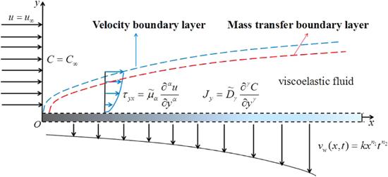
Figure 1. Schematic of viscoelastic incompressible liquid food flowing through a permeable plate. |
3. Implicit numerical method
4. Algorithm analysis
4.1. Mesh independence
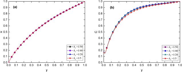
Figure 2. Comparison of $u$ and $C$ with different space step size ${h}_{x}$ with $x=0.8,$ $t=1,$ $\alpha =0.8,$ $\gamma =0.7,$ $\tilde{R{\rm{e}}}=4,$ $\tilde{Sc}=4,$ ${C}_{g}=6.18,$ $k=-5\times {10}^{-3},$ ${n}_{1}=2,$ ${n}_{2}=3,$ ${h}_{y}=1/50,$ $\tau =1/50.$ |
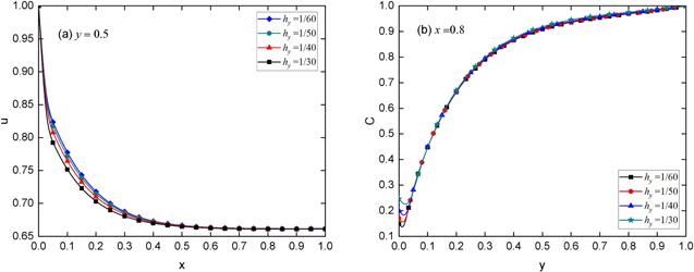
Figure 3. Comparison of $u$ and $C$ with different space step size ${h}_{y}$ with $t=1,$ $\alpha =0.8,$ $\gamma =0.7,$ $\mathop{R{\rm{e}}}\limits^{\sim }=4,$ $\mathop{Sc}\limits^{\sim }=4,$ ${C}_{g}=6.18,$ $k=-5\times {10}^{-3},$ ${n}_{1}=2,$ ${n}_{2}=3,$ ${h}_{x}=1/40,$ $\tau =1/40.$ |
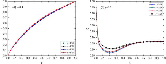
Figure 4. Comparison of $u$ and $C$ with different time step size $\tau $ with $t=1,$ $\alpha =0.8,$ $\gamma =0.7,$ $\mathop{R{\rm{e}}}\limits^{\sim }=4,$ $\mathop{S{\rm{c}}}\limits^{\sim }=4,$ ${C}_{g}=6.18,$ $k=-5\times {10}^{-3},$ ${n}_{1}=2,$ ${n}_{2}=3,$ ${h}_{x}=1/40,$ ${h}_{y}=1/50.$ |
4.2. Accuracy and convergence
4.2.1. Example 1
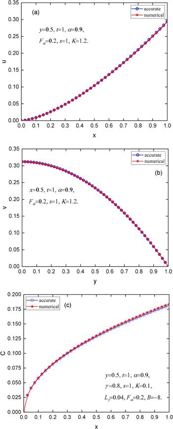
Figure 5. Numerical solution and exact solution of $u,$ $v$ and $C$ with ${h}_{x}=1/40,$ ${h}_{y}=1/50$ and $\tau =1/40.$ |
Table 1. The numerical errors using the difference approximation ( |
| ${h}_{x}$ | ${h}_{y}$ | $\tau $ | ${\parallel {e}^{k}\parallel }_{\max }$ |
|---|---|---|---|
| $1/40$ | $1/40$ | $1/40$ | 2.1068e-04 |
| $1/80$ | $1/80$ | $1/80$ | 1.0726e-04 |
| $1/160$ | $1/160$ | $1/160$ | 5.3961e-05 |
| $1/200$ | $1/200$ | $1/200$ | 4.3193e-05 |
Table 2. The numerical errors using the difference approximation ( |
| ${h}_{x}$ | ${h}_{y}$ | $\tau $ | ${\parallel {\varepsilon }^{k}\parallel }_{\max }$ |
|---|---|---|---|
| $1/40$ | $1/40$ | $1/40$ | 5.3991e-03 |
| $1/80$ | $1/80$ | $1/80$ | 2.9427e-03 |
| $1/160$ | $1/160$ | $1/160$ | 1.5850e-03 |
| $1/200$ | $1/200$ | $1/200$ | 1.2975e-03 |
4.3. Comparison with other method
4.3.1. Example 2
Table 3. Comparisons between G-L algorithm and L1 algorithm with $t=1.$ |
| $(\alpha ,{F}_{\alpha })$ | ${h}_{x}={h}_{y}=\tau $ | $u$ of G-L algorithm | $u$ of L1 algorithm | CPU time of G-L algorithm | CPU time of L1 algorithm |
|---|---|---|---|---|---|
| $(0.9,0.2)$ | $1/40$ | 3.7089e-03 | 3.7380e-03 | 4.143 650 | 4.017 354 |
| $1/80$ | 3.8034e-03 | 3.8185e-03 | 52.166 716 | 51.791 007 | |
| $1/160$ | 3.8535e-03 | 3.8612e-03 | 923.833 059 | 975.019 377 | |
| $(0.8,0.4)$ | $1/40$ | 3.6876e-03 | 3.7343e-03 | 4.481 455 | 3.984 641 |
| $1/80$ | 3.7917e-03 | 3.8156e-03 | 54.090 153 | 51.002 836 | |
| $1/160$ | 3.8474e-03 | 3.8593e-03 | 928.049 600 | 954.880 134 | |
| $(0.7,0.6)$ | $1/40$ | 3.6731e-03 | 3.7271e-03 | 3.992 131 | 3.975 566 |
| $1/80$ | 3.7838e-03 | 3.8110e-03 | 52.689 535 | 50.739 646 | |
| $1/160$ | 3.8431e-03 | 3.8566e-03 | 983.034 463 | 1006.366 636 |
5. Results and discussion
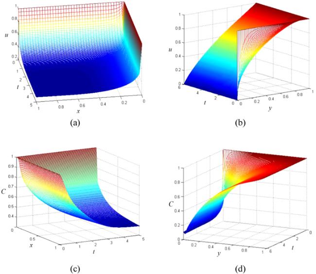
Figure 6. Comparison of $u$ and $C$ with different $t$ for $\alpha =0.8,$ $\gamma =0.7,$ $\mathop{R{\rm{e}}}\limits^{\sim }=4,$ $\mathop{Sc}\limits^{\sim }=4,$ ${C}_{g}=6.18,$ $k=-5\times {10}^{-5},$ ${n}_{1}=2,$ ${n}_{2}=3:$ (a) $y=0.2;$ (b) $x=0.4;$ (c) $y=0.2;$ (d) $x=0.4.$ |
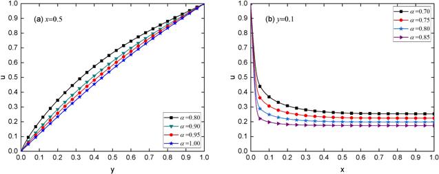
Figure 7. Comparison of $u$ with varying $\alpha $ for $t=1,$ $\tilde{R{\rm{e}}}=4,$ $k=-5\times {10}^{-4},$ ${n}_{1}=2,$ ${n}_{2}=3.$ |
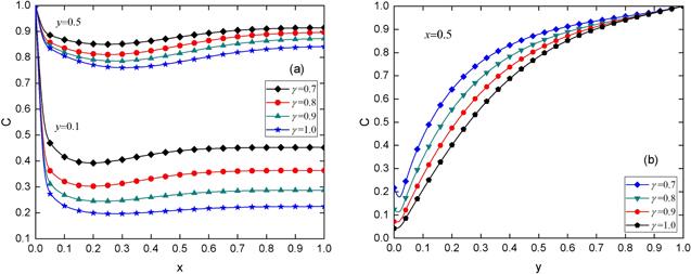
Figure 8. Comparison of $C$ with different $\gamma $ for $t=1,$ $\alpha =0.8,$ $\mathop{R{\rm{e}}}\limits^{\sim }=4,$ $\mathop{Sc}\limits^{\sim }=4,$ ${C}_{g}=6.18,$ $k=-5\times {10}^{-{\rm{4}}},$ ${n}_{1}=2,$ ${n}_{2}=3.$ |
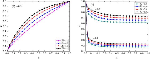
Figure 9. Comparison of $u$ with varying $\mathop{R{\rm{e}}}\limits^{\sim }$ for $t=1,$ $\alpha =0.8,$ $k=-5\times {10}^{-4},$ ${n}_{1}=2,$ ${n}_{2}=3.$ |
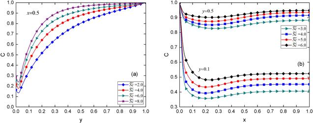
Figure 10. Comparison of $C$ with different $\mathop{Sc}\limits^{\sim }$ for $t=1,$ $\alpha =0.8,$ $\gamma =0.7,$ $\mathop{R{\rm{e}}}\limits^{\sim }=4,$ ${C}_{g}=6.18,$ $k=-5\times {10}^{-{\rm{4}}},$ ${n}_{1}=2,$ ${n}_{2}=3.$ |

Figure 11. Comparison of $C$ with different $k$ for $y=0.06,$ $t=3,$ $\alpha =0.8,$ $\gamma =0.7,$ $\mathop{R{\rm{e}}}\limits^{\sim }=4,$ ${n}_{1}=2,$ ${n}_{2}=3.$ |

Figure 12. Comparison of experimental data from [60] with our results to test the method and the model. |
6. Conclusions
| 1. An increase in fractional-order $\alpha $ brings about a decrease in the horizontal velocity. | |
| 2. Anomalous diffusion weakens the mass transfer; therefore, the concentration decreases by increasing the fractional derivative $\gamma .$ | |
| 3. With an increase in the generalized Reynolds number, the boundary layer thickness reduces, while the fluid velocity increases. | |
| 4. When the generalized Schmidt number rises, the thickness of the concentration boundary layer drops, and the fluid concentration increases. | |
| 5. It is also worth noting that the concentration suddenly decreases slightly near the wall and then gradually increases with an increase in $y.$ |