


| • | Tree operators $\begin{eqnarray}\begin{array}{rcl}{O}_{1}^{u} & = & {\left({\bar{Q}}_{\alpha }{u}_{\beta }\right)}_{V-A}{\left({\bar{u}}_{\beta }{b}_{\alpha }\right)}_{V-A},\\ {O}_{2}^{u} & = & {\left({\bar{Q}}_{\alpha }{u}_{\alpha }\right)}_{V-A}{\left({\bar{u}}_{\beta }{b}_{\beta }\right)}_{V-A}.\end{array}\end{eqnarray}$ |
| • | QCD penguin operators $\begin{eqnarray}\begin{array}{rcl}{O}_{3} & = & {\left({\bar{Q}}_{\alpha }{b}_{\alpha }\right)}_{V-A}\displaystyle \sum _{q^{\prime} }{\left(\bar{q}{{\prime} }_{\beta }q{{\prime} }_{\beta }\right)}_{V-A},\\ {O}_{4} & = & {\left({\bar{Q}}_{\alpha }{b}_{\beta }\right)}_{V-A}\displaystyle \sum _{q^{\prime} }{\left(\bar{q}{{\prime} }_{\beta }q{{\prime} }_{\alpha }\right)}_{V-A},\\ {O}_{5} & = & {\left({\bar{Q}}_{\alpha }{b}_{\alpha }\right)}_{V-A}\displaystyle \sum _{q^{\prime} }{\left(\bar{q}{{\prime} }_{\beta }q{{\prime} }_{\beta }\right)}_{V+A},\\ {O}_{6} & = & {\left({\bar{Q}}_{\alpha }{b}_{\beta }\right)}_{V-A}\displaystyle \sum _{q^{\prime} }{\left(\bar{q}{{\prime} }_{\beta }q{{\prime} }_{\alpha }\right)}_{V+A}.\end{array}\end{eqnarray}$ |
| • | Electroweak penguin operators $\begin{eqnarray}\begin{array}{rcl}{O}_{7} & = & \displaystyle \frac{3}{2}{\left({\bar{Q}}_{\alpha }{b}_{\alpha }\right)}_{V-A}\displaystyle \sum _{q^{\prime} }{e}_{q^{\prime} }{\left(\bar{q}{{\prime} }_{\beta }q{{\prime} }_{\beta }\right)}_{V+A},\\ {O}_{8} & = & \displaystyle \frac{3}{2}{\left({\bar{Q}}_{\alpha }{b}_{\beta }\right)}_{V-A}\displaystyle \sum _{q^{\prime} }{e}_{q^{\prime} }{\left(\bar{q}{{\prime} }_{\beta }q{{\prime} }_{\alpha }\right)}_{V+A},\\ {O}_{9} & = & \displaystyle \frac{3}{2}{\left({\bar{Q}}_{\alpha }{b}_{\alpha }\right)}_{V-A}\displaystyle \sum _{q^{\prime} }{e}_{q^{\prime} }{\left(\bar{q}{{\prime} }_{\beta }q{{\prime} }_{\beta }\right)}_{V-A},\\ {O}_{10} & = & \displaystyle \frac{3}{2}{\left({\bar{Q}}_{\alpha }{b}_{\beta }\right)}_{V-A}\displaystyle \sum _{q^{\prime} }{e}_{q^{\prime} }{\left(\bar{q}{{\prime} }_{\beta }q{{\prime} }_{\alpha }\right)}_{V-A},\end{array}\end{eqnarray}$ |
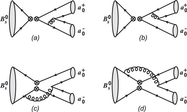
Figure 1. Leading order Feynman diagrams for ${B}_{s}^{0}\to {a}_{0}^{+}{a}_{0}^{-}$ decays in the PQCD formalism. |
| a | (a)For the heavy ${B}_{d}^{0}$ and ${B}_{s}^{0}$ mesons, the wave functions and the distribution amplitudes, and the decay constants are same as those utilized in [39], but with the updated lifetimes ${\tau }_{{B}_{d}^{0}}=1.52$ ps and ${\tau }_{{B}_{s}^{0}}=1.509$ ps [40]. It is worth mentioning that, due to its highly small effects, namely, the power-suppressed 1/mB contributions to B decays in final states with energetic light particles [10, 41], the high twist contributions from the B meson wave function in the considered pure annihilation channels have to be left for future studies associated with the precise measurements. For recent development about the B meson wave function and/or distribution amplitude, please see references, e.g. [41–46] for detail. |
| b | (b)For the considered light scalar a0 and ${K}_{0}^{* }$ states, the decay constants and the Gegenbauer moments in the distribution amplitudes2(2It is necessary to mention that we firstly adopt the asymptotic form of the twist-3 distribution amplitudes φS and φT(T3A) in the numerical calculations here as usual [33, 47]. And then we will estimate the effects in this work arising from the twist-3 distribution amplitudes with inclusion of the Gegenbauer polynomials(T3G) in S2 later. It is noted that only the T3G form in S2 is available currently [48].) have been derived at the normalization scale μ = 1 GeV in the QCD sum rule method [33]: $\begin{eqnarray}{\bar{f}}_{\kappa }=0.340\pm 0.020\,\mathrm{GeV},\,{f}_{\kappa }=0.050\pm 0.003\,\mathrm{GeV},\end{eqnarray}$ $\begin{eqnarray}{B}_{1}=-0.92\pm 0.11,\quad {B}_{3}=0.15\pm 0.09;\end{eqnarray}$ $\begin{eqnarray}{\bar{f}}_{{a}_{0}(980)}=0.365\pm 0.020\,\mathrm{GeV},\,{f}_{{a}_{0}(980)}\sim 0.0011\,\mathrm{GeV},\end{eqnarray}$ $\begin{eqnarray}{B}_{1}=-0.93\pm 0.10,\quad {B}_{3}=0.14\pm 0.08;\end{eqnarray}$ $\begin{eqnarray}\begin{array}{rcl}{\bar{f}}_{{K}_{0}^{* }(1430)} & = & \left\{\begin{array}{ll}-0.300\pm 0.030\,\mathrm{GeV}, & \\ 0.445\pm 0.050\,\mathrm{GeV}, & \end{array}\right.\\ {f}_{{K}_{0}^{* }(1430)} & = & \left\{\begin{array}{ll}-{0.044}_{-0.005}^{+0.004}\,\mathrm{GeV}, & \,({\rm{S}}1)\\ {0.066}_{-0.008}^{+0.007}\,\mathrm{GeV}; & \,({\rm{S}}2)\end{array}\right.\end{array}\end{eqnarray}$ $\begin{eqnarray}{B}_{1}=\left\{\begin{array}{ll}0.58\pm 0.07, & \\ -0.57\pm 0.13, & \end{array}\right.\quad {B}_{3}=\left\{\begin{array}{ll}-1.20\pm 0.08, & \,({\rm{S}}1)\\ -0.42\pm 0.22; & \,({\rm{S}}2)\end{array}\right.\end{eqnarray}$ $\begin{eqnarray}\begin{array}{rcl}{\bar{f}}_{{a}_{0}(1450)} & = & \left\{\begin{array}{ll}-0.280\pm 0.030\,\mathrm{GeV}, & \\ 0.460\pm 0.050\,\mathrm{GeV}, & \end{array}\right.\\ {f}_{{a}_{0}(1450)} & = & \left\{\begin{array}{ll}\sim -0.0009\,\mathrm{GeV}, & \,({\rm{S}}1)\\ {0.0014}_{-0.0001}^{+0.0002}\,\mathrm{GeV}; & \,({\rm{S}}2)\end{array}\right.\end{array}\end{eqnarray}$ $\begin{eqnarray}{B}_{1}=\left\{\begin{array}{ll}0.89\pm 0.20, & \\ -0.58\pm 0.12, & \end{array}\right.\quad {B}_{3}=\left\{\begin{array}{ll}-1.38\pm 0.18, & \,({\rm{S}}1)\\ -0.49\pm 0.15. & \,({\rm{S}}2)\end{array}\right..\end{eqnarray}$ Note that the scale-dependent scalar decay constant ${\bar{f}}_{S}$ and the vector decay constant fS are related with each other through the following relation [33], $\begin{eqnarray}{\bar{f}}_{S}={\mu }_{S}{f}_{S}=\displaystyle \frac{{m}_{S}}{{m}_{{q}_{2}}(\mu )-{m}_{{q}_{1}}(\mu )}{f}_{S},\end{eqnarray}$ in which mS is the mass of the scalar meson, and ${m}_{{q}_{2}}$ and ${m}_{{q}_{1}}$ are the running quark masses. It is worth pointing out that for the a0 states, the isospin symmetry breaking effects from the u and d quark masses are considered. Therefore, the running quark masses for the strange quark and the nonstrange light quarks can be read as ms = 0.128 GeV, md = 0.006 GeV, and mu = 0.003 GeV, respectively, which are translated from those at the $\overline{\mathrm{MS}}$ scale μ ≈ 2 GeV [40]. For the masses of the a0 and ${K}_{0}^{* }$ states, the values mκ = 0.824 GeV, ${m}_{{a}_{0}(980)}=0.980\,\mathrm{GeV}$, ${m}_{{K}_{0}^{* }(1430)}=1.425\,\mathrm{GeV}$, and ${m}_{{a}_{0}(1450)}=1.474$ GeV will be adopted in the numerical calculations3(3As inferred from the Review of Particle Physics [24], the considered scalar a0 and ${K}_{0}^{* }$ states are also with finite widths. Generally speaking, the width effect could change the numerical results with different extent [49, 50]. In principle, we should consider the width effect to make relevant predictions more precise. However, it is unfortunate that the distribution amplitudes for the considered S-wave resonance states with the constrained parameters, e.g. Gegenbauer moments, are currently unavailable. Therefore, we have to leave the width effect in this work for future investigations elsewhere.). |
| c | (c)For the CKM matrix elements, we also adopt the Wolfenstein parametrization at leading order, but with the updated parameters A = 0.836, λ = 0.22453, $\bar{\rho }={0.122}_{-0.017}^{+0.018}$, and $\bar{\eta }={0.355}_{-0.011}^{+0.012}$ [40]. |
| a | (a)For the considered ${B}_{d}^{0}\to {K}_{0}^{* +}{K}_{0}^{* -}$ decays, the CP-averaged branching ratios presented in [35, 39] could be reproduced in this work but with slight differences, which are mainly because of the updated parameters such as the values of the CKM matrix elements, the ${B}_{d}^{0}$ meson lifetime, and the running quark masses of the light quarks. As aforementioned, the ${B}_{d}^{0}\to {K}^{+}{K}^{-}$ decay has been measured experimentally and the decay rate is read as 7.8 ± 1.5 × 10⁻⁸ [24], which confirmed the PQCD calculation, that is, ${1.56}_{-0.52}^{+0.56}\times {10}^{-7}$ [28] about this channel theoretically. As the counterpart with the same quark structure in the scalar sector, the ${B}_{d}^{0}\to {K}_{0}^{* +}{K}_{0}^{* -}$ modes with large decay rates in the order of 10−6 predicted with the same PQCD formalism could be examined at the LHCb and/or Belle-II experiments in the (near) future. The confirmation from the experimental side would help explore the inner structure especially for the scalar ${K}_{0}^{* }(1430)$ meson. |
| b | (b)For the ${B}_{s}^{0}\to {a}_{0}^{+}{a}_{0}^{-}$ modes, they have the same quark structure as that of the measured one ${B}_{s}^{0}\to {\pi }^{+}{\pi }^{-}$, whose decay rate is read as 7.0 ± 1.0 × 10⁻⁷ [24] and agrees well with the prediction about the decay rate ${5.10}_{-1.89}^{+2.26}\times {10}^{-7}$ [28] in the PQCD approach within theoretical errors. Therefore, the large ${B}_{s}^{0}\to {a}_{0}^{+}{a}_{0}^{-}$ decay rates in the order of 10−5 could be accessed with much more probabilities experimentally with respect to those of the ${B}_{d}^{0}\to {K}_{0}^{* +}{K}_{0}^{* -}$ ones. Furthermore, (i)Recently, the ${B}_{s}^{0}\to {a}_{0}{\left(980\right)}^{+}{a}_{0}{\left(980\right)}^{-}$ mode has been investigated in the PQCD approach by Liang and Yu [37]. However, it is a bit strange that the CP-averaged branching ratio of the ${B}_{s}^{0}\to {a}_{0}{\left(980\right)}^{+}{a}_{0}{\left(980\right)}^{-}$ channel is predicted as small as ${5.17}_{-1.94}^{+2.36}\times {10}^{-6}$. In fact, as naively estimated from the ${B}_{s}^{0}\to {\pi }^{+}{\pi }^{-}$ decay rate, the ${B}_{s}^{0}\to {a}_{0}{\left(980\right)}^{+}{a}_{0}{\left(980\right)}^{-}$ branching ratio could be, as far as the central values are concerned, $| \tfrac{{\bar{f}}_{{a}_{0}(980)}}{{f}_{\pi }}{| }^{2}\cdot | \tfrac{{\bar{f}}_{{a}_{0}(980)}}{{f}_{\pi }}{| }^{2}\cdot {Br}{\left({B}_{s}^{0}\to {\pi }^{+}{\pi }^{-}\right)}_{\mathrm{Exp}}\sim 4.34\times {10}^{-5}$ and $| \tfrac{{\bar{f}}_{{a}_{0}(980)}}{{f}_{\pi }}{| }^{2}\cdot | \tfrac{{\bar{f}}_{{a}_{0}(980)}}{{f}_{\pi }}{| }^{2}\cdot {Br}{\left({B}_{s}^{0}\to {\pi }^{+}{\pi }^{-}\right)}_{\mathrm{PQCD}}\sim 3.16\,\times \,{10}^{-5}$ singly induced by the decay constants fπ = 0.13 GeV and ${\bar{f}}_{{a}_{0}(980)}=0.365\,\mathrm{GeV}$, apart from the possible enhancement arising from the asymmetric behavior of the only odd terms involved in the leading twist distribution amplitude of the scalar meson. (ii)We study the ${B}_{s}^{0}\to {a}_{0}{\left(1450\right)}^{+}{a}_{0}{\left(1450\right)}^{-}$ decay in two scenarios within the PQCD framework for the first time. The predicted branching ratios are large around 10−5 and are expected to be tested in the near future at LHCb and/or Belle-II experiments. The understanding of the scalar a0(1450) meson could provide useful information to uncover the nature of the ${K}_{0}^{* }(1430)$ meson through the SU(3) flavor symmetry (breaking) effects, and vice versa. |
| c | (c)In light of the large theoretical errors, a precise ratio of the related branching ratios would be more interested because, generally speaking, the theoretical errors resulted from the hadronic inputs could be cancelled to a great extent. Therefore, we define the following ratios to be measured at the relevant experiments of B meson decays, which would help to study the QCD dynamics, even the decay mechanism of these considered pure annihilation decays. $\begin{eqnarray}\begin{array}{l}{R}_{{sd}}^{{a}_{0}(980)/\kappa }\equiv \displaystyle \frac{{Br}\left({B}_{s}^{0}\to {a}_{0}{\left(980\right)}^{+}{a}_{0}{\left(980\right)}^{-}\right)}{{Br}({B}_{d}^{0}\to {\kappa }^{+}{\kappa }^{-})}\\ =\ {9.30}_{-0.33}^{+0.40}{\left({\omega }_{B}\right)}_{-0.31}^{+0.42}{\left({B}_{m}\right)}_{-0.17}^{+0.16}{\left({\bar{f}}_{M}\right)}_{-0.46}^{+0.44}(V)[{9.30}_{-0.67}^{+0.75}],\end{array}\end{eqnarray}$ $\begin{eqnarray}\begin{array}{l}{R}_{{sd}}^{{a}_{0}(1450)/{K}_{0}^{* }(1430)}\equiv \displaystyle \frac{{Br}\left({B}_{s}^{0}\to {a}_{0}{\left(1450\right)}^{+}{a}_{0}{\left(1450\right)}^{-}\right)}{{Br}\left({B}_{d}^{0}\to {K}_{0}^{* }{\left(1430\right)}^{+}{K}_{0}^{* }{\left(1430\right)}^{-}\right)}\\ =\,\left\{\begin{array}{ll}{18.28}_{-0.11}^{+0.00}{\left({\omega }_{B}\right)}_{-4.34}^{+4.12}{\left({B}_{m}\right)}_{-0.56}^{+0.52}{\left({\bar{f}}_{M}\right)}_{-0.78}^{+0.80}(V)[{18.28}_{-4.45}^{+4.23}], & \,({\rm{S}}1)\\ {14.49}_{-0.63}^{+0.75}{\left({\omega }_{B}\right)}_{-0.86}^{+1.54}{\left({B}_{m}\right)}_{-1.16}^{+0.25}{\left({\bar{f}}_{M}\right)}_{-0.47}^{+0.51}(V)[{14.49}_{-1.64}^{+1.80}]. & \,({\rm{S}}2)\end{array}\right.\end{array}\,\end{eqnarray}$ $\begin{eqnarray}\begin{array}{l}{R}_{d}^{{\rm{S}}1/{\rm{S}}2}\left({K}_{0}^{* }\left(1430\right)\right)\equiv \displaystyle \frac{{Br}{\left({B}_{d}^{0}\to {K}_{0}^{* }{\left(1430\right)}^{+}{K}_{0}^{* }{\left(1430\right)}^{-}\right)}_{{\rm{S}}1}}{{Br}{\left({B}_{d}^{0}\to {K}_{0}^{* }{\left(1430\right)}^{+}{K}_{0}^{* }{\left(1430\right)}^{-}\right)}_{{\rm{S}}2}}\\ =\ {1.26}_{-0.22}^{+0.23}{\left({\omega }_{B}\right)}_{-0.37}^{+0.65}{\left({B}_{m}\right)}_{-0.14}^{+0.07}{\left({\bar{f}}_{M}\right)}_{-0.02}^{+0.02}(V)[{1.26}_{-0.45}^{+0.69}],\end{array}\end{eqnarray}$ $\begin{eqnarray}\begin{array}{l}{R}_{s}^{{\rm{S}}1/{\rm{S}}2}({a}_{0}(1450))\equiv \displaystyle \frac{{Br}{\left({B}_{s}^{0}\to {a}_{0}{\left(1450\right)}^{+}{a}_{0}{\left(1450\right)}^{-}\right)}_{{\rm{S}}1}}{{Br}{\left({B}_{s}^{0}\to {a}_{0}{\left(1450\right)}^{+}{a}_{0}{\left(1450\right)}^{-}\right)}_{{\rm{S}}2}}\\ =\ {1.59}_{-0.34}^{+0.36}{\left({\omega }_{B}\right)}_{-0.10}^{+0.07}{\left({B}_{m}\right)}_{-0.01}^{+0.01}{\left({\bar{f}}_{M}\right)}_{-0.01}^{+0.00}(V)[{1.59}_{-0.35}^{+0.37}],\end{array}\end{eqnarray}$ $\begin{eqnarray}\begin{array}{l}{R}_{d,{\rm{S}}1}^{{K}_{0}^{* }(1430)/\kappa }\equiv \displaystyle \frac{{Br}{\left({B}_{d}^{0}\to {K}_{0}^{* }{\left(1430\right)}^{+}{K}_{0}^{* }{\left(1430\right)}^{-}\right)}_{{\rm{S}}1}}{{Br}({B}_{d}^{0}\to {\kappa }^{+}{\kappa }^{-})}\\ =\ {1.08}_{-0.06}^{+0.06}{\left({\omega }_{B}\right)}_{-0.16}^{+0.20}{\left({B}_{m}\right)}_{-0.17}^{+0.18}{\left({\bar{f}}_{M}\right)}_{-0.00}^{+0.01}(V)[{1.08}_{-0.24}^{+0.28}],\end{array}\end{eqnarray}$ $\begin{eqnarray}\begin{array}{l}{R}_{d,{\rm{S}}2}^{{K}_{0}^{* }(1430)/\kappa }\equiv \displaystyle \frac{{Br}{\left({B}_{d}^{0}\to {K}_{0}^{* }{\left(1430\right)}^{+}{K}_{0}^{* }{\left(1430\right)}^{-}\right)}_{{\rm{S}}2}}{{Br}({B}_{d}^{0}\to {\kappa }^{+}{\kappa }^{-})}\\ =\ {0.86}_{-0.09}^{+0.12}{\left({\omega }_{B}\right)}_{-0.19}^{+0.18}{\left({B}_{m}\right)}_{-0.18}^{+0.27}{\left({\bar{f}}_{M}\right)}_{-0.04}^{+0.02}(V)[{0.86}_{-0.28}^{+0.35}],\end{array}\end{eqnarray}$ $\begin{eqnarray}\begin{array}{l}{R}_{s,{\rm{S}}1}^{{a}_{0}(1450)/{a}_{0}(980)}\equiv \displaystyle \frac{{Br}{\left({B}_{s}^{0}\to {a}_{0}{\left(1450\right)}^{+}{a}_{0}{\left(1450\right)}^{-}\right)}_{{\rm{S}}1}}{{Br}\left({B}_{s}^{0}\to {a}_{0}{\left(980\right)}^{+}{a}_{0}{\left(980\right)}^{-}\right)}\\ =\ {2.13}_{-0.22}^{+0.19}{\left({\omega }_{B}\right)}_{-0.30}^{+0.16}{\left({B}_{m}\right)}_{-0.43}^{+0.46}{\left({\bar{f}}_{M}\right)}_{-0.00}^{+0.00}(V)[{2.13}_{-0.57}^{+0.52}],\end{array}\end{eqnarray}$ $\begin{eqnarray}\begin{array}{l}{R}_{s,{\rm{S}}2}^{{a}_{0}(1450)/{a}_{0}(980)}\equiv \displaystyle \frac{{Br}{\left({B}_{s}^{0}\to {a}_{0}{\left(1450\right)}^{+}{a}_{0}{\left(1450\right)}^{-}\right)}_{{\rm{S}}2}}{{Br}\left({B}_{s}^{0}\to {a}_{0}{\left(980\right)}^{+}{a}_{0}{\left(980\right)}^{-}\right)}\\ =\ {1.34}_{-0.15}^{+0.19}{\left({\omega }_{B}\right)}_{-0.24}^{+0.20}{\left({B}_{m}\right)}_{-0.28}^{+0.30}{\left({\bar{f}}_{M}\right)}_{-0.00}^{+0.01}(V)[{1.34}_{-0.40}^{+0.41}].\end{array}\end{eqnarray}$ Of course, it is found that the uncertainties in some of the above ratios are not small, for example, ${R}_{d}^{{\rm{S}}1/{\rm{S}}2}({K}_{0}^{* }(1430))={1.26}_{-0.45}^{+0.69}$ in equation ( |
| d | (d)Another eight more interesting ratios could be obtained and are expected to be examined at the future experiments, if we take the already measured ${B}_{d}^{0}\to {K}^{+}{K}^{-}$ and ${B}_{s}^{0}\to {\pi }^{+}{\pi }^{-}$ decays as referenced channels. By combing the branching fractions of the ${B}_{d}^{0}\to {K}^{+}{K}^{-}$ and ${B}_{s}^{0}\to {\pi }^{+}{\pi }^{-}$ decays from both of the PQCD predictions [28] and the experimental measurements [24] sides, and the decay rates of the ${B}_{d}^{0}\to {K}_{0}^{* +}{K}_{0}^{* -}$ and ${B}_{s}^{0}\to {a}_{0}^{+}{a}_{0}^{-}$ modes in this work, they are read as follows, $\begin{eqnarray}{R}_{d,\mathrm{Exp}}^{\kappa /K}\equiv \displaystyle \frac{{Br}{\left({B}_{d}^{0}\to {\kappa }^{+}{\kappa }^{-}\right)}_{\mathrm{PQCD}}}{{Br}{\left({B}_{d}^{0}\to {K}^{+}{K}^{-}\right)}_{\mathrm{Exp}}}={36.41}_{-10.70}^{+11.55},\end{eqnarray}$ $\begin{eqnarray}\begin{array}{rcl}{R}_{d,\mathrm{Exp}}^{{K}_{0}^{* }(1430)/K} & \equiv & \displaystyle \frac{{Br}{\left({B}_{d}^{0}\to {K}_{0}^{* }{\left(1430\right)}^{+}{K}_{0}^{* }{\left(1430\right)}^{-}\right)}_{\mathrm{PQCD}}}{{Br}{\left({B}_{d}^{0}\to {K}^{+}{K}^{-}\right)}_{\mathrm{Exp}}}\\ & = & \left\{\begin{array}{ll}{39.49}_{-11.55}^{+11.48}, & \,({\rm{S}}1)\\ {31.41}_{-18.08}^{+22.57}; & \,({\rm{S}}2)\end{array}\right.\end{array}\end{eqnarray}$ $\begin{eqnarray}{R}_{d,\mathrm{Th}}^{\kappa /K}\equiv \displaystyle \frac{{Br}{\left({B}_{d}^{0}\to {\kappa }^{+}{\kappa }^{-}\right)}_{\mathrm{PQCD}}}{{Br}{\left({B}_{d}^{0}\to {K}^{+}{K}^{-}\right)}_{\mathrm{PQCD}}}={18.21}_{-2.63}^{+2.83},\end{eqnarray}$ $\begin{eqnarray}\begin{array}{rcl}{R}_{d,\mathrm{Th}}^{{K}_{0}^{* }(1430)/K} & \equiv & \displaystyle \frac{{Br}{\left({B}_{d}^{0}\to {K}_{0}^{* }{\left(1430\right)}^{+}{K}_{0}^{* }{\left(1430\right)}^{-}\right)}_{\mathrm{PQCD}}}{{Br}{\left({B}_{d}^{0}\to {K}^{+}{K}^{-}\right)}_{\mathrm{PQCD}}}\\ & = & \left\{\begin{array}{ll}{19.74}_{-2.82}^{+2.62}, & \,({\rm{S}}1)\\ {15.71}_{-7.63}^{+7.97}; & \,({\rm{S}}2)\end{array}\right.\end{array}\end{eqnarray}$ and $\begin{eqnarray}\begin{array}{rcl}{R}_{s,\mathrm{Exp}}^{{a}_{0}(980)/\pi } & \equiv & \displaystyle \frac{{Br}{\left({B}_{s}^{0}\to {a}_{0}{\left(980\right)}^{+}{a}_{0}{\left(980\right)}^{-}\right)}_{\mathrm{PQCD}}}{{Br}{\left({B}_{s}^{0}\to {\pi }^{+}{\pi }^{-}\right)}_{\mathrm{Exp}}}\\ & = & {37.18}_{-10.85}^{+13.07},\end{array}\end{eqnarray}$ $\begin{eqnarray}\begin{array}{rcl}{R}_{s,\mathrm{Exp}}^{{a}_{0}(1450)/\pi } & \equiv & \displaystyle \frac{{Br}{\left({B}_{s}^{0}\to {a}_{0}{\left(1450\right)}^{+}{a}_{0}{\left(1450\right)}^{-}\right)}_{\mathrm{PQCD}}}{{Br}{\left({B}_{s}^{0}\to {\pi }^{+}{\pi }^{-}\right)}_{\mathrm{Exp}}}\\ & = & \left\{\begin{array}{ll}{80.43}_{-39.43}^{+42.82}, & \,({\rm{S}}1)\\ {50.71}_{-28.38}^{+32.54}; & \,({\rm{S}}2)\end{array}\right.\end{array}\end{eqnarray}$ $\begin{eqnarray}\begin{array}{rcl}{R}_{s,\mathrm{Th}}^{{a}_{0}(980)/\pi } & \equiv & \displaystyle \frac{{Br}{\left({B}_{s}^{0}\to {a}_{0}{\left(980\right)}^{+}{a}_{0}{\left(980\right)}^{-}\right)}_{\mathrm{PQCD}}}{{Br}{\left({B}_{s}^{0}\to {\pi }^{+}{\pi }^{-}\right)}_{\mathrm{PQCD}}}\\ & = & {51.76}_{-2.54}^{+2.86},\end{array}\end{eqnarray}$ $\begin{eqnarray}\begin{array}{rcl}{R}_{s,\mathrm{Th}}^{{a}_{0}(1450)/\pi } & \equiv & \displaystyle \frac{{Br}{\left({B}_{s}^{0}\to {a}_{0}{\left(1450\right)}^{+}{a}_{0}{\left(1450\right)}^{-}\right)}_{\mathrm{PQCD}}}{{Br}{\left({B}_{s}^{0}\to {\pi }^{+}{\pi }^{-}\right)}_{\mathrm{PQCD}}}\\ & = & \left\{\begin{array}{ll}{110.39}_{-33.75}^{+23.58}, & \,({\rm{S}}1)\\ {69.61}_{-27.87}^{+20.88}. & \,({\rm{S}}2)\end{array}\right..\end{array}\end{eqnarray}$ These large values of the above ratios with still large theoretical errors could be easily tested when the related samples are collected with good precision experimentally. |
| e | (e)As mentioned in the above, the isospin symmetry breaking effects from the u and d quark masses have been considered in the ${B}_{s}^{0}\to {a}_{0}^{+}{a}_{0}^{-}$ decays. Therefore, the factorizable annihilation decay amplitudes are not exact zero, which can be seen clearly from the numerical results as shown in the tables 1 and 2 in both scenarios S1 and S2. However, they are still tiny and could be neglected safely. It means that the contributions to the pure annihilation decays considered in this work are absolutely from the nonfactorizable annihilation decay amplitudes. It is noticed that, relative to the ${B}_{d}^{0}\to {K}^{+}{K}^{-}$ and ${B}_{s}^{0}\to {\pi }^{+}{\pi }^{-}$ decays, the antisymmetric QCD behavior of the leading twist distribution amplitude could make the destructive interferences in the pseudoscalar sector become the constructive ones in the scalar sector to the nonfactorizable annihilation diagrams between the figure 1(c) with hard gluon radiating from light d(s) quark and the figure 1(d) with hard gluon radiating from heavy anti-b quark, which eventually result in the large CP-averaged decay rates of the considered decays, as presented in the equations ( |
Table 1. The factorization decay amplitudes(in units of 10−3 GeV3) in S1 of the pure annihilation ${B}_{d}^{0}\to {K}_{0}^{* +}{K}_{0}^{* -}$ and ${B}_{s}^{0}\to {a}_{0}^{+}{a}_{0}^{-}$ decays in the PQCD approach, where only the central values are quoted for clarifications. |
| Modes | Anfa(T3A) | Afa(T3A) |
|---|---|---|
| ${B}_{d}^{0}\to {K}_{0}^{* }{(800)}^{+}{K}_{0}^{* }{(800)}^{-}$ | − 0.610 − i1.974 | 0.0008 + i0.0004 |
| ${B}_{d}^{0}\to {K}_{0}^{* }{(1430)}^{+}{K}_{0}^{* }{(1430)}^{-}$ | 1.877 − i2.658 | 0.001 + i0.003 |
| ${B}_{s}^{0}\to {a}_{0}{\left(980\right)}^{+}{a}_{0}{\left(980\right)}^{-}$ | 6.892 + i1.325 | 0.00003 − i0.002 |
| ${B}_{s}^{0}\to {a}_{0}{\left(1450\right)}^{+}{a}_{0}{\left(1450\right)}^{-}$ | − 1.588 + i10.057 | − 0.006 + i0.002 |
Table 2. Similar to table 1 but in S2 for the ${B}_{d}^{0}\to {K}_{0}^{* }{\left(1430\right)}^{+}{K}_{0}^{* }{\left(1430\right)}^{-}$ and ${B}_{s}^{0}\to {a}_{0}{\left(1450\right)}^{+}{a}_{0}{\left(1450\right)}^{-}$ decays. |
| Modes | Anfa(T3A) | Afa(T3A) | Anfa(T3G) | Afa(T3G) |
|---|---|---|---|---|
| ${B}_{d}^{0}\to {K}_{0}^{* }{(1430)}^{+}{K}_{0}^{* }{(1430)}^{-}$ | − 1.940 + i0.188 | − 0.0005 − i0.0006 | − 1.617 + i1.571 | − 0.028 + i0.762 |
| ${B}_{s}^{0}\to {a}_{0}{\left(1450\right)}^{+}{a}_{0}{\left(1450\right)}^{-}$ | 5.038 − i6.778 | − 0.002 + i0.000 06 | 4.851 − i6.812 | 0.006 + i0.003 |
| a | (a)For the ${B}_{d}^{0}\to {K}_{0}^{* +}{K}_{0}^{* -}$ decays, $\begin{eqnarray}\begin{array}{l}{{ \mathcal A }}_{\mathrm{dir}}({B}_{d}^{0}\to {\kappa }^{+}{\kappa }^{-})\,=\ {15.5}_{-0.6}^{+0.0}{\left({\omega }_{B}\right)}_{-5.4}^{+3.7}{\left({B}_{m}\right)}_{-0.0}^{+0.0}{\left({\bar{f}}_{{K}_{0}^{* }}\right)}_{-0.8}^{+0.7}(V)[{15.5}_{-5.5}^{+3.8}]\,\times \ {10}^{-2},\end{array}\end{eqnarray}$ $\begin{eqnarray}\begin{array}{l}{{ \mathcal A }}_{\mathrm{mix}}({B}_{d}^{0}\to {\kappa }^{+}{\kappa }^{-})\,=\ -{80.4}_{-0.2}^{+0.1}{\left({\omega }_{B}\right)}_{-3.8}^{+3.5}{\left({B}_{m}\right)}_{-0.0}^{+0.0}{\left({\bar{f}}_{{K}_{0}^{* }}\right)}_{-3.3}^{+3.8}(V)[-{80.4}_{-5.0}^{+5.2}]\,\times \ {10}^{-2};\end{array}\end{eqnarray}$ and $\begin{eqnarray}\begin{array}{l}{{ \mathcal A }}_{\mathrm{dir}}\left({B}_{d}^{0}\to {K}_{0}^{* }{\left(1430\right)}^{+}{K}_{0}^{* }{\left(1430\right)}^{-}\right)\,=\ \left\{\begin{array}{l}-{73.9}_{-0.0}^{+0.8}{\left({\omega }_{B}\right)}_{-4.7}^{+4.6}{\left({B}_{m}\right)}_{-0.2}^{+0.0}{\left({\bar{f}}_{{K}_{0}^{* }}\right)}_{-2.3}^{+2.5}(V)[-{73.9}_{-5.2}^{+5.3}]\times {10}^{-2}({\rm{S}}1),\\ {21.4}_{-0.8}^{+0.6}{\left({\omega }_{B}\right)}_{-2.7}^{+8.8}{\left({B}_{m}\right)}_{-0.7}^{+0.0}{\left({\bar{f}}_{{K}_{0}^{* }}\right)}_{-0.8}^{+0.9}(V)[{21.4}_{-3.0}^{+8.9}]\times {10}^{-2}({\rm{S}}2);\end{array}\right.\end{array}\end{eqnarray}$ $\begin{eqnarray}\begin{array}{l}{{ \mathcal A }}_{\mathrm{mix}}\left({B}_{d}^{0}\to {K}_{0}^{* }{\left(1430\right)}^{+}{K}_{0}^{* }{\left(1430\right)}^{-}\right)\,=\,\left\{\begin{array}{l}-{39.6}_{-6.3}^{+5.6}{\left({\omega }_{B}\right)}_{-5.9}^{+6.1}{\left({B}_{m}\right)}_{-0.0}^{+0.3}{\left({\bar{f}}_{{K}_{0}^{* }}\right)}_{-5.3}^{+5.7}(V)[-{39.6}_{-10.1}^{+10.1}]\times {10}^{-2}({\rm{S}}1),\\ -{97.5}_{-0.2}^{+0.1}{\left({\omega }_{B}\right)}_{-0.4}^{+2.5}{\left({B}_{m}\right)}_{-0.2}^{+0.0}{\left({\bar{f}}_{{K}_{0}^{* }}\right)}_{-0.4}^{+0.4}(V)[-{97.5}_{-0.6}^{+2.5}]\times {10}^{-2}({\rm{S}}2);\end{array}\right.\end{array}\end{eqnarray}$ |
| b | (b)For the ${B}_{s}^{0}\to {a}_{0}^{+}{a}_{0}^{-}$ decays, $\begin{eqnarray}\begin{array}{l}{{ \mathcal A }}_{\mathrm{dir}}\left({B}_{s}^{0}\to {a}_{0}{\left(980\right)}^{+}{a}_{0}{\left(980\right)}^{-}\right)=-{0.7}_{-0.0}^{+0.0}{\left({\omega }_{B}\right)}_{-0.1}^{+0.5}{\left({B}_{m}\right)}_{-0.0}^{+0.0}\,\times \ {\left({\bar{f}}_{{a}_{0}}\right)}_{-0.0}^{+0.1}(V)[-{0.7}_{-0.1}^{+0.5}]\times {10}^{-2},\end{array}\end{eqnarray}$ $\begin{eqnarray}\begin{array}{l}{{ \mathcal A }}_{\mathrm{mix}}\left({B}_{s}^{0}\to {a}_{0}{\left(980\right)}^{+}{a}_{0}{\left(980\right)}^{-}\right)={13.6}_{-0.1}^{+0.0}{\left({\omega }_{B}\right)}_{-1.0}^{+1.0}{\left({B}_{m}\right)}_{-0.0}^{+0.0}\,\times \ {\left({\bar{f}}_{{a}_{0}}\right)}_{-0.4}^{+0.5}(V)[{13.6}_{-1.1}^{+1.1}]\times {10}^{-2},\end{array}\end{eqnarray}$ $\begin{eqnarray}\begin{array}{l}{{ \mathcal A }}_{{\rm{\Delta }}{{\rm{\Gamma }}}_{s}}\left({B}_{s}^{0}\to {a}_{0}{\left(980\right)}^{+}{a}_{0}{\left(980\right)}^{-}\right)={99.1}_{-0.0}^{+0.0}{\left({\omega }_{B}\right)}_{-0.2}^{+0.1}{\left({B}_{m}\right)}_{-0.0}^{+0.0}{\left({\bar{f}}_{{a}_{0}}\right)}_{-0.1}^{+0.0}(V)\,\times \,[{99.1}_{-0.2}^{+0.1}]\times {10}^{-2};\end{array}\end{eqnarray}$ and $\begin{eqnarray}\begin{array}{l}{{ \mathcal A }}_{\mathrm{dir}}\left({B}_{s}^{0}\to {a}_{0}{\left(1450\right)}^{+}{a}_{0}{\left(1450\right)}^{-}\right)\,=\,\left\{\begin{array}{l}{9.6}_{-0.8}^{+0.9}{\left({\omega }_{B}\right)}_{-1.2}^{+0.9}{\left({B}_{m}\right)}_{-0.1}^{+0.0}{\left({\bar{f}}_{{a}_{0}}\right)}_{-0.3}^{+0.3}(V)[{9.6}_{-1.5}^{+1.3}]\times {10}^{-2}({\rm{S}}1),\\ {1.4}_{-0.0}^{+0.1}{\left({\omega }_{B}\right)}_{-0.5}^{+0.4}{\left({B}_{m}\right)}_{-0.0}^{+0.1}{\left({\bar{f}}_{{a}_{0}}\right)}_{-0.0}^{+0.1}(V)[{1.4}_{-0.5}^{+0.4}]\times {10}^{-2}({\rm{S}}2);\end{array}\right.\end{array}\end{eqnarray}$ $\begin{eqnarray}\begin{array}{l}{{ \mathcal A }}_{\mathrm{mix}}\left({B}_{s}^{0}\to {a}_{0}{\left(1450\right)}^{+}{a}_{0}{\left(1450\right)}^{-}\right)\,=\ \left\{\begin{array}{l}{14.0}_{-0.1}^{+0.0}{\left({\omega }_{B}\right)}_{-1.6}^{+1.3}{\left({B}_{m}\right)}_{-0.0}^{+0.0}{\left({\bar{f}}_{{a}_{0}}\right)}_{-0.4}^{+0.5}(V)[{14.0}_{-1.7}^{+1.4}]\times {10}^{-2}({\rm{S}}1),\\ {7.2}_{-0.0}^{+0.1}{\left({\omega }_{B}\right)}_{-0.7}^{+0.6}{\left({B}_{m}\right)}_{-0.0}^{+0.0}{\left({\bar{f}}_{{a}_{0}}\right)}_{-0.2}^{+0.3}(V)[{7.2}_{-0.7}^{+0.7}]\times {10}^{-2}({\rm{S}}2);\end{array}\right.\end{array}\end{eqnarray}$ $\begin{eqnarray}\begin{array}{l}{{ \mathcal A }}_{{\rm{\Delta }}{{\rm{\Gamma }}}_{s}}\left({B}_{s}^{0}\to {a}_{0}{\left(1450\right)}^{+}{a}_{0}{\left(1450\right)}^{-}\right)\,=\ \left\{\begin{array}{l}{98.6}_{-0.1}^{+0.0}{\left({\omega }_{B}\right)}_{-0.1}^{+0.0}{\left({B}_{m}\right)}_{-0.0}^{+0.0}{\left({\bar{f}}_{{a}_{0}}\right)}_{-0.1}^{+0.0}(V)[{98.6}_{-0.2}^{+0.0}]\times {10}^{-2}({\rm{S}}1),\\ {99.7}_{-0.0}^{+0.0}{\left({\omega }_{B}\right)}_{-0.0}^{+0.1}{\left({B}_{m}\right)}_{-0.0}^{+0.0}{\left({\bar{f}}_{{a}_{0}}\right)}_{-0.0}^{+0.0}(V)[{99.7}_{-0.0}^{+0.1}]\times {10}^{-2}({\rm{S}}2),\end{array}\right.\end{array}\end{eqnarray}$ |
| • | It is clear to see that these predicted CP violations are generally insensitive to the variation of the scalar decay constant ${\bar{f}}_{M}(M={a}_{0},\ {K}_{0}^{* })$. The underlying reason is that the decay amplitudes of the considered decays are nearly proportional to the scalar decay constant, due to the vanishing vector decay constant (see equations ( $\begin{eqnarray}\begin{array}{l}{\phi }_{S}(x,\mu )=\displaystyle \frac{3}{\sqrt{6}}x(1-x)\,\times \,\left\{{f}_{S}(\mu )+{\bar{f}}_{S}(\mu )\displaystyle \sum _{m=1}^{\infty }{B}_{m}(\mu ){C}_{m}^{3/2}(2x-1)\right\},\end{array}\end{eqnarray}$ where fS(μ) and ${\bar{f}}_{S}(\mu )$, Bm(μ), and ${C}_{m}^{3/2}(t)$ are the vector and the scalar decay constants, the Gegenbauer moments, and the Gegenbauer polynomials, respectively, and the asymptotic forms of the twist-3 distribution amplitudes of the scalar a0 and ${K}_{0}^{* }$ mesons. While, the CP asymmetries of the ${B}_{d}^{0}\to {K}_{0}^{* }{\left(1430\right)}^{+}{K}_{0}^{* }{\left(1430\right)}^{-}$ decays are more sensitive to the ${\bar{f}}_{{K}_{0}^{* }(1430)}$ than those of the ${B}_{s}^{0}\to {a}_{0}{\left(1450\right)}^{+}{a}_{0}{\left(1450\right)}^{-}$ ones to the ${\bar{f}}_{{a}_{0}(1450)}$. The fact is that the isospin symmetry breaking effect from the u and d quark masses leads to the tiny and negligible vector decay constant ${f}_{{a}_{0}(1450)}$, i.e. equation ( |
| • | It is easy to find that, apart from the ${{ \mathcal A }}_{\mathrm{dir}}{\left({B}_{s}^{0}\to {a}_{0}{\left(980\right)}^{+}{a}_{0}{\left(980\right)}^{-}\right)}_{{\rm{S}}1}$ and ${{ \mathcal A }}_{\mathrm{dir}}{B}_{s}^{0}\to {a}_{0}{\left(1450\right)}^{+}{a}_{0}{{\left(1450\right)}^{-}}_{{\rm{S}}2}$ with few percent, the rest CP-violating asymmetries for the considered pure annihilation decays of ${B}_{d}^{0}\to {K}_{0}^{* +}{K}_{0}^{* -}$ and ${B}_{s}^{0}\to {a}_{0}^{+}{a}_{0}^{-}$ in the PQCD approach are large, which means that the contributions from the penguin diagrams are generally sizable. To see this point explicitly, we present the decay amplitudes classified as the tree diagrams and the penguin ones, respectively, in the tables 3–4, where only the central values are quoted for clarifications. Then it is expected that these predictions of the CP violations, associated with the predicted large decay rates, could be confronted with the relevant experiments at LHCb and/or Belle-II in the (near) future. Of course, the ${{ \mathcal A }}_{\mathrm{dir}}{\left({B}_{s}^{0}\to {a}_{0}{\left(980\right)}^{+}{a}_{0}{\left(980\right)}^{-}\right)}_{{\rm{S}}1}$ and ${{ \mathcal A }}_{\mathrm{dir}}{B}_{s}^{0}\to {a}_{0}{\left(1450\right)}^{+}{a}_{0}{{\left(1450\right)}^{-}}_{{\rm{S}}2}$ are too small to be measured easily in the near future, though the corresponding branching ratios are as large as 10−5. |
Table 3. The tree and penguin decay amplitudes(in units of 10−3 GeV3) in S1 of the pure annihilation ${B}_{d}^{0}\to {K}_{0}^{* +}{K}_{0}^{* -}$ and ${B}_{s}^{0}\to {a}_{0}^{+}{a}_{0}^{-}$ decays in the PQCD approach, where the results in the parentheses are the corresponding amplitudes of the ${\bar{B}}_{d}^{0}\to {K}_{0}^{* +}{K}_{0}^{* -}$ and ${\bar{B}}_{s}^{0}\to {a}_{0}^{+}{a}_{0}^{-}$ decays, and only the central values are considered for clarifications. |
| Modes | Tree diagrams(T3A) | Penguin diagrams(T3A) |
|---|---|---|
| ${B}_{d}^{0}\to {K}_{0}^{* }{\left(800\right)}^{+}{K}_{0}^{* }{(800)}^{-}$ | $\begin{array}{c}0.551-{\rm{i}}\ 1.920\ \\ (-1.615+{\rm{i}}\ 1.176)\end{array}$ | $\begin{array}{c}-1.160-{\rm{i}}\ 0.054\ \\ (-0.779-{\rm{i}}\ 0.861)\end{array}$ |
| ${B}_{d}^{0}\to {K}_{0}^{* }{\left(1430\right)}^{+}{K}_{0}^{* }{(1430)}^{-}$ | $\begin{array}{c}1.633-{\rm{i}}\ 1.433\ \\ (-2.169+{\rm{i}}\ 0.126)\end{array}$ | $\begin{array}{c}0.245-{\rm{i}}\ 1.222\ \\ (1.040-{\rm{i}}\ 0.687)\end{array}$ |
| ${B}_{s}^{0}\to {a}_{0}{\left(980\right)}^{+}{a}_{0}{\left(980\right)}^{-}$ | $\begin{array}{c}-0.013-{\rm{i}}\ 0.504\ \\ (-0.300+{\rm{i}}\ 0.406)\end{array}$ | $\begin{array}{c}6.906+{\rm{i}}\ 1.827\ \\ (6.906+{\rm{i}}\ 1.827)\end{array}$ |
| ${B}_{s}^{0}\to {a}_{0}{\left(1450\right)}^{+}{a}_{0}{\left(1450\right)}^{-}$ | $\begin{array}{c}0.738-{\rm{i}}\ 0.619\ \\ (-0.963+{\rm{i}}\ 0.035)\end{array}$ | $\begin{array}{c}-2.332+{\rm{i}}\ 10.678\ \\ (-2.332+{\rm{i}}\ 10.678)\end{array}$ |
Table 4. Similar to table 3 but in S2 for the ${B}_{d}^{0}\to {K}_{0}^{* }{\left(1430\right)}^{+}{K}_{0}^{* }{\left(1430\right)}^{-}$ and ${B}_{s}^{0}\to {a}_{0}{\left(1450\right)}^{+}{a}_{0}{\left(1450\right)}^{-}$ decays. |
| Modes | Tree diagrams(T3A) | Penguin diagrams(T3A) | Tree diagrams(T3G) | Penguin diagrams(T3G) |
|---|---|---|---|---|
| ${B}_{d}^{0}\to {K}_{0}^{* }{(1430)}^{+}{K}_{0}^{* }{(1430)}^{-}$ | $\begin{array}{c}-1.081-{\rm{i}}\ 1.178\ \\ (0.129+{\rm{i}}\ 1.593)\end{array}$ | $\begin{array}{c}-0.859+{\rm{i}}\ 1.365\ \\ (-1.574+{\rm{i}}\ 0.352)\end{array}$ | $\begin{array}{c}-0.566+{\rm{i}}\ 0.658\ \\ (0.850-{\rm{i}}\ 0.171)\end{array}$ | $\begin{array}{c}-1.079+{\rm{i}}\ 1.675\ \\ (-1.949+{\rm{i}}\ 0.415)\end{array}$ |
| ${B}_{s}^{0}\to {a}_{0}{\left(1450\right)}^{+}{a}_{0}{\left(1450\right)}^{-}$ | $\begin{array}{c}-0.328-{\rm{i}}\ 0.048\ \\ (0.229+{\rm{i}}\ 0.239)\end{array}$ | $\begin{array}{c}5.364-{\rm{i}}\ 6.730\ \\ (5.364-{\rm{i}}\ 6.730)\end{array}$ | $\begin{array}{c}-0.097+{\rm{i}}\ 0.188\ \\ (0.192-{\rm{i}}\ 0.088)\end{array}$ | $\begin{array}{c}4.954-{\rm{i}}\ 6.998\ \\ (4.954-{\rm{i}}\ 6.998)\end{array}$ |
| • | The large decay rates in the order of 10−6 and 10−5 have been obtained in the PQCD calculations for the pure annihilation ${B}_{d}^{0}\to {K}_{0}^{* +}{K}_{0}^{* -}$ and ${B}_{s}^{0}\to {a}_{0}^{+}{a}_{0}^{-}$ decays, respectively, but which suffer from large theoretical uncertainties mainly arising from the hadronic parameters of the scalar a0 and ${K}_{0}^{* }$ mesons, such as the Gegenbauer moments, the scalar decay constants, etc. Undoubtedly, these large predictions in the PQCD approach could be examined at the LHCb and/or Belle-II experiments in the (near) future. |
| • | Except for the ${{ \mathcal A }}_{\mathrm{dir}}{\left({B}_{s}^{0}\to {a}_{0}{\left(980\right)}^{+}{a}_{0}{\left(980\right)}^{-}\right)}_{{\rm{S}}1}$ and ${{ \mathcal A }}_{\mathrm{dir}}{\left({B}_{s}^{0}\to {a}_{0}{\left(1450\right)}^{+}{a}_{0}{\left(1450\right)}^{-}\right)}_{{\rm{S}}2}$ in the order of 1%, the large CP-violating asymmetries could be found in the rest ${B}_{d}^{0}\to {K}_{0}^{* +}{K}_{0}^{* -}$ and ${B}_{s}^{0}\to {a}_{0}^{+}{a}_{0}^{-}$ modes. These asymmetries could also be tested in the future measurements with the help of the predicted large branching ratios. |
| • | The ${B}_{d}^{0}\to {K}_{0}^{* }{\left(1430\right)}^{+}{K}_{0}^{* }{\left(1430\right)}^{-}$ and ${B}_{s}^{0}\,\to {a}_{0}{\left(1450\right)}^{+}{a}_{0}{\left(1450\right)}^{-}$ decays are investigated in S2 with two different kinds of twist-3 distribution amplitudes, i.e. the asymptotic form and the Gegenbauer polynomial form. And the latter form could change the strong phases evidently, and subsequently change the CP-violating asymmetries apparently. |
| • | The unknown inner structure or QCD dynamics of the scalar states demands the reliable studies from the experimental examinations, or in the nonperturbative techniques, for example, Lattice QCD. The clear understanding about the QCD dynamics of the scalars must constrain the errors of the predictions in the PQCD approach of the pure annihilation modes in this work, which would provide opportunities to shed light on the mechanism of the annihilation decays. |