


1. Introduction
The study of the structure of hyperons, which contain strange quarks, via their electromagnetic form factors (EMFFs) is crucial for a deep understanding of the nonperturbative quantum chromodynamics (QCD) effect whereby quarks are bounded by baryons [1–5]. As discussed in [6–8], EMFFs are crucial experimental observables of baryons, which are intimately related to their internal structure and dynamics. In the last few decades, there has been great progress in the study of baryon EMFFs, especially for nucleons, in both the timelike [9–20] and spacelike regions [21–31]. For example, in [32] the nucleon form factors and the N-Δ(1232) transitions were theoretically investigated using the framework of a constituent quark model, where the effect of the π meson cloud is also considered. However, since hyperons cannot be targets, hyperon EMFFs in the spacelike region have hardly been experimentally measured. In the timelike region, the Beijing Spectrometer III (BESIII) collaboration has investigated the Σ hyperon EMFFs using the reaction ${e}^{+}{e}^{-}\to {{\rm{\Sigma }}}^{+}{\bar{{\rm{\Sigma }}}}^{-}$ and ${e}^{+}{e}^{-}\to {{\rm{\Sigma }}}^{-}{\bar{{\rm{\Sigma }}}}^{+}$ [4, 33]. The effective form factors ∣Geff∣ of Σ+ and Σ− and the ratios of the Σ+ electric and magnetic form factors ∣GE/GM∣ were obtained [4] from the high-precision Born cross-sections determined for the two abovementioned reactions for center-of-mass energies from 2.3864 to 3.02GeV.
Very recently, the EMFFs of hyperons have been investigated in the timelike region through ${e}^{+}{e}^{-}\to Y\bar{Y}$ (Y is the hyperon) reaction [5], where the $Y\bar{Y}$ final state interactions were taken into account, and the EMFFs in the timelike region were calculated for the Λ, Σ, and ξ hyperons based on the one-photon exchange approximation of the elementary reaction mechanism. In [2], the timelike EMFFs of hyperons were accurately reproduced within a relativistic quark model. In addition, the Σ hyperon EMFFs have been calculated using lattice QCD [34], the light-cone sum rule (LCSR) [35], and chiral perturbative theory (ChPT) [36]. In addition to these, the vector-meson dominance (VMD) model is a very successful approach for the study of nucleon electromagnetic form factors, in both the spacelike and timelike regions [37–39]. Within a modified VMD model, in [1] the EMFFs of the Λ hyperon have been studied in the timelike region using the ${e}^{+}{e}^{-}\to {\rm{\Lambda }}\bar{{\rm{\Lambda }}}$ reaction, where the contributions from φ and ω mesons and their excited states were included. It was found that the VMD model was able to simultaneously describe the effective form factor and also the electromagnetic form factor ratio of the Λ hyperon.
In this work, based on the recent measurements of the ${e}^{+}{e}^{-}\to {{\rm{\Sigma }}}^{+}{\bar{{\rm{\Sigma }}}}^{-}$ and ${e}^{+}{e}^{-}\to {{\rm{\Sigma }}}^{-}{\bar{{\rm{\Sigma }}}}^{+}$ reactions, we aim to determine the parameters of the VMD model by fitting them to the experimental data of ∣Geff∣ of Σ+ and Σ−. We have included the contributions of the ρ, ω and φ mesons. The ratios ∣GE/GM∣ of Σ+ are then estimated with the model parameters, which are comparable to those obtained using other theoretical calculations.
This article is organized as follows: the formalism of the Σ hyperon form factors in the VMD model are shown in the following section. In section 3 , we introduce effective form factors and the method that analytically continues the expressions of the form factors from the timelike region to the spacelike region. The numerical results of the timelike form factors of the Σ+ and Σ− hyperons and the ratios ∣GE/GM∣ of Σ+ and Σ− are presented in section 4 , followed by a short summary in the final section.
2. Theoretical formalism
In this paper, we study the EMFFs of Σ+ and Σ− using the VMD model. As in [1], we first introduce the electromagnetic current of the Σ hyperon with a half spin in terms of the Dirac form factor F1(Q2) and the Pauli form factors F2(Q2) as $\begin{eqnarray}{J}^{\mu }={\gamma }^{u}{F}_{1}({Q}^{2})+{\rm{i}}\displaystyle \frac{{\sigma }^{\mu \nu }{q}_{\nu }}{2{m}_{{\rm{\Sigma }}}}{F}_{2}({Q}^{2}),\end{eqnarray}$ where F1 and F2 are functions of the squared momentum transfer Q2 = − q2. In the VMD model, the Dirac and Pauli form factors are parameterized into two parts. One is the intrinsic three-quark structure described by the form factor g(Q2) [39], the other is the meson cloud, which is used to describe the interaction between a bare baryon and a photon through the intermediate isovector ρ meson and the isoscalar ω and φ mesons [37]. Following [37–39], F1 and F2 can be decomposed into ${F}_{i}={F}_{i}^{S}+{F}_{i}^{V}$ , where FiS and FiV are the isoscalar and isovector components of the form factors, respectively. The Dirac and Pauli form factors of Σ+ and Σ− are then easily obtained without considering the total decay widths of the vector mesons, as follows: $\begin{eqnarray}\begin{array}{l}{F}_{1{{\rm{\Sigma }}}^{+}}^{S}\left({Q}^{2}\right)=\frac{1}{2}{g}_{1}\left({Q}^{2}\right)\\ \ \ \ \times \left[\left(1-{\beta }_{\omega }-{\beta }_{\phi }\right)+{\beta }_{\omega }\frac{{m}_{\omega }^{2}}{{m}_{\omega }^{2}+{Q}^{2}}+{\beta }_{\phi }\frac{{m}_{\phi }^{2}}{{m}_{\phi }^{2}+{Q}^{2}}\right],\end{array}\end{eqnarray}$ $\begin{eqnarray}\begin{array}{l}{F}_{1{{\rm{\Sigma }}}^{+}}^{V}\left({Q}^{2}\right)=\displaystyle \frac{1}{2}{g}_{1}\left({Q}^{2}\right)\\ \ \ \ \times \,\left[\left(1-{\beta }_{\rho }\right)+{\beta }_{\rho }\displaystyle \frac{{m}_{\rho }^{2}}{{m}_{\rho }^{2}+{Q}^{2}}\right],\end{array}\end{eqnarray}$ $\begin{eqnarray}\begin{array}{l}{F}_{2{{\rm{\Sigma }}}^{+}}^{S}\left({Q}^{2}\right)=\displaystyle \frac{1}{2}{g}_{1}\left({Q}^{2}\right)\\ \ \ \ \times \,\left[\left(2{\mu }_{{{\rm{\Sigma }}}^{+}}-2-{\alpha }_{\phi }-{\alpha }_{\rho }\right)\displaystyle \frac{{m}_{\omega }^{2}}{{m}_{\omega }^{2}+{Q}^{2}}+{\alpha }_{\phi }\displaystyle \frac{{m}_{\phi }^{2}}{{m}_{\phi }^{2}+{Q}^{2}}\right],\end{array}\end{eqnarray}$ $\begin{eqnarray}{F}_{2{{\rm{\Sigma }}}^{+}}^{V}\left({Q}^{2}\right)=\displaystyle \frac{1}{2}{g}_{1}\left({Q}^{2}\right)\left[{\alpha }_{\rho }\displaystyle \frac{{m}_{\rho }^{2}}{{m}_{\rho }^{2}+{Q}^{2}}\right],\end{eqnarray}$ $\begin{eqnarray}\begin{array}{l}{F}_{1{{\rm{\Sigma }}}^{-}}^{S}\left({Q}^{2}\right)=\displaystyle \frac{1}{2}{g}_{2}\left({Q}^{2}\right)\\ \ \ \ \times \,\left[\left(-1-{\beta }_{\omega }-{\beta }_{\phi }\right)+{\beta }_{\omega }\displaystyle \frac{{m}_{\omega }^{2}}{{m}_{\omega }^{2}+{Q}^{2}}+{\beta }_{\phi }\displaystyle \frac{{m}_{\phi }^{2}}{{m}_{\phi }^{2}+{Q}^{2}}\right],\end{array}\end{eqnarray}$ $\begin{eqnarray}{F}_{1{{\rm{\Sigma }}}^{-}}^{V}\left({Q}^{2}\right)=\displaystyle \frac{1}{2}{g}_{2}\left({Q}^{2}\right)\left[\left(-1-{\beta }_{\rho }\right)+{\beta }_{\rho }\displaystyle \frac{{m}_{\rho }^{2}}{{m}_{\rho }^{2}+{Q}^{2}}\right],\end{eqnarray}$ $\begin{eqnarray}\begin{array}{l}{F}_{2{{\rm{\Sigma }}}^{-}}^{S}\left({Q}^{2}\right)=\frac{1}{2}{g}_{2}\left({Q}^{2}\right)\\ \ \ \ \times \left[\left(2{\mu }_{{{\rm{\Sigma }}}^{-}}+2-{\alpha }_{\phi }-{\alpha }_{\rho }\right)\frac{{m}_{\omega }^{2}}{{m}_{\omega }^{2}+{Q}^{2}}+{\alpha }_{\phi }\frac{{m}_{\phi }^{2}}{{m}_{\phi }^{2}+{Q}^{2}}\right],\end{array}\end{eqnarray}$ $\begin{eqnarray}{F}_{2{{\rm{\Sigma }}}^{-}}^{V}\left({Q}^{2}\right)=\displaystyle \frac{1}{2}{g}_{2}\left({Q}^{2}\right)\left[{\alpha }_{\rho }\displaystyle \frac{{m}_{\rho }^{2}}{{m}_{\rho }^{2}+{Q}^{2}}\right],\end{eqnarray}$ where we take the intrinsic form factor g(Q2) as a dipole form $\begin{eqnarray}{g}_{1}{({Q}^{2})=(1+{\gamma }_{1}{Q}^{2})}^{-2},\end{eqnarray}$ $\begin{eqnarray}{g}_{2}{({Q}^{2})=(1+{\gamma }_{2}{Q}^{2})}^{-2}.\end{eqnarray}$ This form is consistent with g = 1 at Q2 = 0, and the free model parameters γ1 and γ2 are determined by fitting them to the experimental data.
On the other hand, the observed electric and magnetic form factors, GE and GM, can be expressed in terms of the Dirac and Pauli form factors F1 and F2 by $\begin{eqnarray}{G}_{E}({Q}^{2})={F}_{1}-\tau {F}_{2}={F}_{1}^{S}+{F}_{1}^{V}-\tau ({F}_{2}^{S}+{F}_{2}^{V}),\end{eqnarray}$ $\begin{eqnarray}{G}_{M}({Q}^{2})={F}_{1}+{F}_{2}={F}_{1}^{S}+{F}_{1}^{V}+{F}_{2}^{S}+{F}_{2}^{V},\end{eqnarray}$ where $\tau =\tfrac{{Q}^{2}}{4{M}_{{\rm{\Sigma }}}^{2}}$ in this work. At Q2=0, GM(Q2) defines the value of the magnetic moment of the Σ hyperon, μΣ = GM(0), in natural units, i.e., ${\hat{\mu }}_{{\rm{\Sigma }}}=e/(2{M}_{{\rm{\Sigma }}})$ . To easily compare the magnetic moments of different particle masses, it is usual to express magnetic moments in terms of ${\hat{\mu }}_{N}=e/(2{M}_{N})$ , the nucleon magneton [40, 41]. In this work, we use ${\mu }_{{{\rm{\Sigma }}}^{+}}=3.112$ and ${\mu }_{{{\rm{\Sigma }}}^{-}}=-1.479$ with natural units [40]. In addition, we let mρ=0.775, mω = 0.782, and mφ = 1.019GeV [40].
In equations (2 )–(9 ), βρ, βω, βφ, αφ, and αρ represent the product of a vector–meson–photon coupling constant and a VΣΣ coupling constant. The VΣΣ coupling constants are obtained through an SU(3) flavor symmetry, as in [42], $\begin{eqnarray}{g}_{{\rm{\Sigma }}{\rm{\Sigma }}\omega }={g}_{{BBV}}2{\alpha }_{{BBV}},\end{eqnarray}$ $\begin{eqnarray}{g}_{{\rm{\Sigma }}{\rm{\Sigma }}\phi }=-{g}_{{BBV}}\sqrt{2}\left(2{\alpha }_{{BBV}}-1\right),\end{eqnarray}$ $\begin{eqnarray}{g}_{{\rm{\Sigma }}{\rm{\Sigma }}\rho }={g}_{{BBV}}2{\alpha }_{{BBV}},\end{eqnarray}$ where gBBV = gNNρ = 3.20 and αBBV = 1.15, as used in [42, 43]. We can now easily get gΣΣω = 7.36, gΣΣφ = −5.88, gΣΣρ = 7.36, while the tensor couplings are given by $\begin{eqnarray}{f}_{{\rm{\Sigma }}{\rm{\Sigma }}\phi }={f}_{{NN}\rho }\displaystyle \frac{1}{\sqrt{2}},\,\,\,{f}_{{\rm{\Sigma }}{\rm{\Sigma }}\rho }={f}_{{NN}\rho }\displaystyle \frac{1}{2},\end{eqnarray}$ where fNNρ = gNNρκρ and κρ = 6.1 [42, 43]. Therefore, we can get fΣΣφ = 13.80 and fΣΣρ = 9.76.
In addition, we calculate the Vγ coupling constants following [44–46], $\begin{eqnarray}{{ \mathcal L }}_{V\gamma }=\displaystyle \sum _{V}\displaystyle \frac{{{eM}}_{V}^{2}}{{f}_{V}}{V}_{\mu }{A}^{\mu },\end{eqnarray}$ $\begin{eqnarray}\displaystyle \frac{e}{{f}_{V}}={\left[\displaystyle \frac{3{{\rm{\Gamma }}}_{V\to {e}^{+}{e}^{-}}}{2{\alpha }_{e}\left|{\vec{p}}_{e}\right|}\right]}^{1/2}.\end{eqnarray}$ where αe = e2/(4π) = 1/137 is the fine-structure constant and ${\vec{p}}_{e}$ is the three momentum of the electron in the rest frame of the vector meson. ${{\rm{\Gamma }}}_{V\to {e}^{+}{e}^{-}}$ is the partial decay width of the vector meson when it decays into a e+e− pair. With the experimental values, we now get 1/fρ = 0.200, 1/fω = 0.059, and 1/fφ = 0.075.
Finally, we obtain βρ, βω, βφ, αφ and αρ through $\begin{eqnarray}{\beta }_{V}={g}_{{\rm{\Sigma }}{\rm{\Sigma }}V}\displaystyle \frac{1}{{f}_{V}},\,\,{\alpha }_{V}={f}_{{\rm{\Sigma }}{\rm{\Sigma }}V}\displaystyle \frac{1}{{f}_{V}},\end{eqnarray}$ which are summarized in table 1.
Table 1. Parameters used in this work. |
| Parameter | Value | Parameter | Value |
|---|---|---|---|
| βρ | 0.736 | αρ | 0.976 |
| βφ | −0.441 | αφ | 1.035 |
| βω | 0.434 |
We now explain how the large total width of the ρ meson contributions are implemented. 4() For this purpose, one needs to replace [37] $\begin{eqnarray}\begin{array}{l}\displaystyle \frac{{m}_{\rho }^{2}}{{m}_{\rho }^{2}+{Q}^{2}}\to \\ \displaystyle \frac{{m}_{\rho }^{2}+8{{\rm{\Gamma }}}_{\rho }{m}_{\pi }/\pi }{{m}_{\rho }^{2}+{Q}^{2}+\left(4{m}_{\pi }^{2}+{Q}^{2}\right){{\rm{\Gamma }}}_{\rho }\alpha \left({Q}^{2}\right)/{m}_{\pi }},\end{array}\end{eqnarray}$ where we let Γρ = 149.1, and the average value of mπ = 138.04 MeV [40]. The function α(Q2) is given by $\begin{eqnarray*}\alpha \left({Q}^{2}\right)=\displaystyle \frac{2}{\pi }{\left(\displaystyle \frac{4{m}_{\pi }^{2}+{Q}^{2}}{{Q}^{2}}\right)}^{1/2}\mathrm{ln}\left(\displaystyle \frac{\sqrt{4{m}_{\pi }^{2}+{Q}^{2}}+\sqrt{{Q}^{2}}}{2{m}_{\pi }}\right).\end{eqnarray*}$
The timelike form factors can be obtained from the spacelike form factors by an appropriate analytic continuation. Within the above ingredients, $g\left({q}^{2}\right)$ has the form required for an analytical continuation, $\begin{eqnarray}g\left({q}^{2}\right)={\left(1-\gamma {q}^{2}\right)}^{-2},\end{eqnarray}$ where Q2 = −q2 = q2eiπ. We note that γ has a positive value, hence, g(q2) will be divergent at q2 = 1/γ. To evade this problem, one can restrict $\gamma \gt 1/(4{m}_{{\rm{\Sigma }}}^{2})$ .
3. Numerical results and discussion
In the timelike region, the EMFFs of the hyperons Σ+ and Σ− are experimentally studied via the electron–position annihilation processes. Under the one-photon exchange approximation, the total cross-section of ${e}^{+}{e}^{-}\to Y\bar{Y}$ , where Y is Σ+ or Σ−, can be expressed in terms of the electric and magnetic form factors GE and GM, as described in [47] $\begin{eqnarray}\sigma =\displaystyle \frac{4\pi {\alpha }_{e}^{2}\beta }{3{q}^{2}}{C}_{{\rm{\Sigma }}}\left({\left|{G}_{M}\left({q}^{2}\right)\right|}^{2}+\displaystyle \frac{2{M}_{{\rm{\Sigma }}}^{2}}{{q}^{2}}{\left|{G}_{E}\left({q}^{2}\right)\right|}^{2}\right),\end{eqnarray}$ where $\beta =\sqrt{1-4{M}_{{\rm{\Sigma }}}^{2}/{q}^{2}}$ is a phase-space factor. Here, q2 = s is the invariant mass square of the e+e− system. In addition, the Coulomb correction factor CΣ is given by [47] $\begin{eqnarray}C(y)=\displaystyle \frac{y}{1-{{\rm{e}}}^{-y}},\end{eqnarray}$ with $y=\tfrac{\alpha \pi }{\beta }\tfrac{2{M}_{{\rm{\Sigma }}}}{q}$ .
In general, one can easily obtain the effective form factor Geff(q2) from the total cross-section of the e+e− annihilation process. The effective form factor, Geff(q2), is defined as $\begin{eqnarray}\left|{G}_{\mathrm{eff}}\left({q}^{2}\right)\right|=\sqrt{\displaystyle \frac{2\tau {\left|{G}_{M}\left({q}^{2}\right)\right|}^{2}+{\left|{G}_{E}\left({q}^{2}\right)\right|}^{2}}{1+2\tau }}.\end{eqnarray}$
We then perform a χ2 fit to the experimental data of the effective form factor ∣Geff∣ of Σ+ and Σ− taken from [4]. In the fitting, we only have one free parameter: γ1 for Σ+, and γ2 for Σ−. The fitted parameters are γ1 = 0.46 ± 0.01 GeV−2 and γ2 = 1.18 ± 0.13 GeV−2, with χ2/dof = 2.0 and 1.1, respectively. The corresponding best-fitting results for the effective form factor ∣Geff∣ of Σ+ and Σ− in the energy range 2.3864GeV $\lt \sqrt{s}\lt $ 2.9884 GeV are shown in figure 1 using solid curves. We also show the theoretical band obtained from the above uncertainties of the fitted parameters. The numerical results show that we can give a good description for the experimental data.
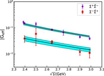
Figure 1. The solid curves represent the theoretical results for the ∣Geff∣ of the Σ+ and Σ− using the fitted parameters. The experimental data for Σ+ and Σ− are taken from [4]. |
From the fitted results of the effective form factors, we can easily obtain the values of $| {G}_{\mathrm{eff}}^{{{\rm{\Sigma }}}^{+}}| /| {G}_{\mathrm{eff}}^{{{\rm{\Sigma }}}^{-}}| $ , which are shown in figure 2. One can see that the ratio is about three in the energy region of $2.4\lt \sqrt{s}\lt 3.0\,\,\mathrm{GeV}$ . The value of three is just the ratio of the incoherent sum of the squared charges of the Σ+ and Σ− valence quarks.
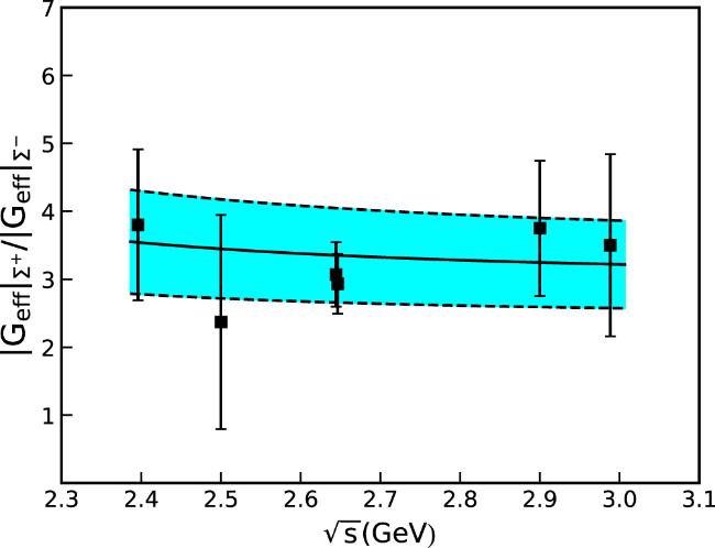
Figure 2. Theoretical results for the ratio of |
Through the vector-meson dominance model, using the fitted parameter γ, one can also easily calculate the ratio of ∣GE∣ and ∣GM∣. This ratio is determined to be one at the mass threshold of a baryon–anti-baryon pair, due to the kinematical restriction. We show our theoretical calculations in figure 3, where the results are obtained with γ1 = 0.46 and γ2 = 1.18. It is found that when the reaction energy $\sqrt{s}$ increases, the ratio of ∣GE∣ and ∣GM∣ for Σ+ slowly decreases, while for the case of Σ−, it is almost flat. Our results here do not adequately explain the experimental data, which show that the ratio is larger than one within uncertainties close to the threshold. This may indicate that there should be also other contributions in that energy region. For example, the electromagnetic form factors should be significantly influenced by the interaction in the final ${\rm{\Sigma }}\bar{{\rm{\Sigma }}}$ system [5]. However, since the experimental and empirical information about the ${\rm{\Sigma }}\bar{{\rm{\Sigma }}}$ final state interaction is so limited, we leave those contributions to further study when more precise data are available.
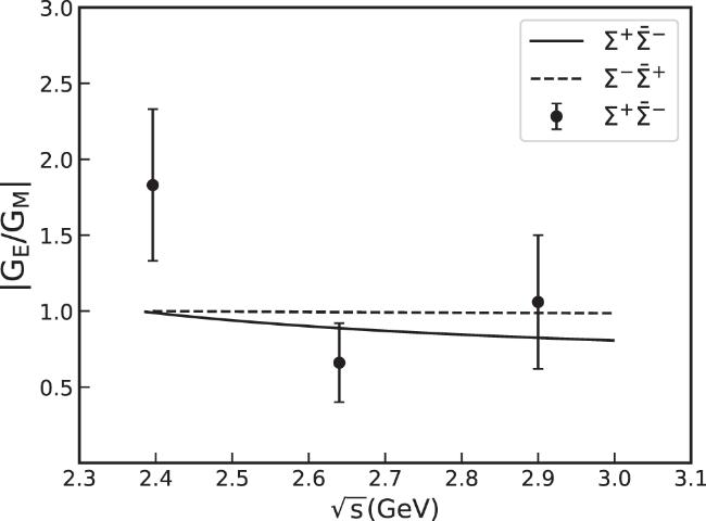
Figure 3. The results for the ratio of ∣GE/GM∣ of the Σ+ and Σ−. The data are for Σ+ and taken from [4]. |
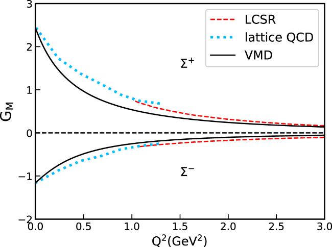
We next pay attention to the EMFFs in the spacelike region, which can be straightforwardly calculated with the parameter γ determined by the experimental measurements in the timelike region. Since the parameterization forms shown in equations (2 )–(9 ) are valid in the low Q2 regime, we calculate GE and GM below Q2 = 3 GeV2, and compare our numerical results with other calculations.
The numerical results for the GM and GE obtained with γ1 = 0.46 and γ2 = 1.18 are shown in figures 4 and 5, respectively. 5() In figure 4, the predictions of the light-cone sum rules [35] and the lattice QCD calculations [34] are also shown for comparison. Our results for the magnetic form factors of Σ+ and Σ− are somewhat quantitatively different from those obtained using other theories. Our results for the magnetic form factor of Σ− are more consistent with other calculations, while for the case of the Σ− electric form factor in figure 5, our results are in disagreement with the ChPT and LCSR calculations. However, our results for the Σ+ are closer to the lattice QCD results described in [34] and the ChPT results in the very low Q2 region. It is expected that these theoretical calculations can be tested by future experiments on the EMFFs of the Σ+ and Σ− hyperons and will thus provide new insights into the complex internal structure of the baryons.

4. Summary
In this work, we have investigated the electromagnetic form factors of the hyperons Σ+ and Σ− within the vector-meson dominance model. The contributions of the ρ, ω and φ mesons were taken into account. The model parameters, γ1 and γ2, were determined using the BESIII experimental data for the timelike effective form factors ∣Geff∣ of Σ+ and Σ−. It was found that the experimental data were able to be reproduced well using only one model parameter. We analytically continued the electromagnetic form factors into the spacelike region and evaluated the spacelike form factors of Σ+ and Σ−. The electromagnetic form factors obtained for the Σ+ and Σ− and their ratio were qualitatively comparable with those of other model calculations, but slightly different quantitatively.
Finally, we would like to stress that the estimations of the Σ form factors in this work, the Λ form factors in [1] and the proton form factors in [37–39] indicate that the vector-meson dominance model is valid for the study of the baryonic electromagnetic form factors. Accurate data for the e+e− → baryon + anti-baryon reaction can be used to improve our knowledge of baryon form factors, which are, at present, poorly known.