


1. Introduction
2. QCD sum rules for the tetraquark and hexaquark molecular states
where $J(x)={J}_{c\bar{c}}(x)$, ${J}_{{cc}}(x)$, ${J}_{\mu }(x)={J}_{\mu }^{{cc}\bar{c}}(x)$, ${J}_{\mu }^{{ccc}}(x)$,
where q = u or d. The color-singlet-color-singlet type currents ${J}_{c\bar{c}}(x)$ and ${J}_{{cc}}(x)$ couple potentially to the scalar hidden-charm and doubly charmed tetraquark molecular states or two-meson scattering states, respectively, the color-singlet-color-singlet-color-singlet type currents ${J}_{\mu }^{{cc}\bar{c}}(x)$ and ${J}_{\mu }^{{ccc}}(x)$ couple potentially to the vector charmed plus hidden-charm and triply charmed hexaquark molecular states or three-meson scattering states, respectively. The currents ${J}_{c\bar{c}}(x)$, Jcc(x), ${J}_{\mu }^{{cc}\bar{c}}(x)$ and ${J}_{\mu }^{{ccc}}(x)$ have the isospins I = 0, 1, $\tfrac{1}{2}$ and $\tfrac{3}{2}$, respectively. In the isospin limit, the currents with the same isospins couple potentially to the hadrons or hadron-systems with almost degenerated masses.
where the subscripts T and H denote the scalar ${D}^{* }{\bar{D}}^{* }$, ${D}^{* }{D}^{* }$ tetraquark molecular states and the vector ${D}^{* }{D}^{* }{\bar{D}}^{* }$, ${D}^{* }{D}^{* }{D}^{* }$ hexaquark molecular states, respectively, and we have used the definitions for the pole residues,
the ${\varepsilon }_{\mu }$ are the polarization vectors of the vector hexaquark molecular states. In [13], we observe that, for the color-singlet-color-singlet type currents, the meson-meson scattering states alone cannot saturate the QCD sum rules, while the tetraquark molecular states alone can saturate the QCD sum rules, the net effects of the two-meson scattering states amount to modifying the pole residues considerably without influencing the predicted masses. In this article, we only take into account the tetraquark and hexaquark molecular states, as the widths of those molecular states, which absorb the contributions of the two-meson or three-meson scattering states, are unknown.
where the Sij(x) and Cij(x) are the full light and heavy quark propagators, respectively,
and ${t}^{n}=\tfrac{{\lambda }^{n}}{2}$, the ${\lambda }^{n}$ is the Gell-Mann matrix [2, 24, 25], we add the subscripts $c\bar{c}$, cc, ${cc}\bar{c}$ and ccc to denote the corresponding currents. In the full light quark propagator, see equation (
The induced currents ${\hat{J}}_{c\bar{c}}(x)$ and ${\hat{J}}_{\mu }^{{cc}\bar{c}}(x)$ have two and four valence quarks, respectively. Such contractions are neglected as an approximation. However, one should bear in mind that such an approximation may lead to a sizeable uncertainty. We will take into account those contributions in the future.
the QCD spectral densities ${\rho }_{T,\mathrm{QCD}}(s)$ are given explicitly in the
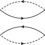
Figure 1. The Feynman diagram for the lowest order contribution for the current ${J}_{c\bar{c}}(x)$, where the solid lines and dashed lines represent the light quarks and heavy quarks, respectively. |
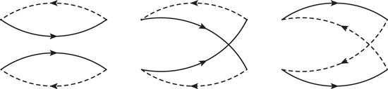
Figure 2. The Feynman diagrams for the lowest order contributions for the current Jcc(x), where the solid lines and dashed lines represent the light quarks and heavy quarks, respectively. |
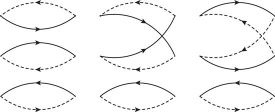
Figure 3. The Feynman diagrams for the lowest order contributions for the current ${J}_{\mu }^{{cc}\bar{c}}(x)$, where the solid lines and dashed lines represent the light quarks and heavy quarks, respectively. |
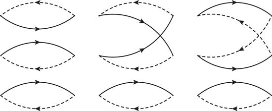
Figure 4. The factorizable Feynman diagrams in the color space for the lowest order contributions for the current ${J}_{\mu }^{{ccc}}(x)$, where the solid lines and dashed lines represent the light quarks and heavy quarks, respectively. |
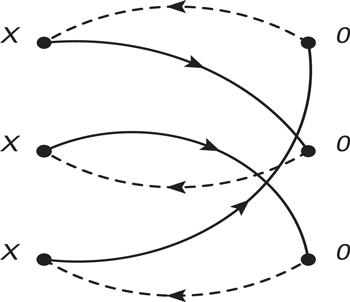
Figure 5. The nonfactorizable Feynman diagrams in the color space for the lowest order contributions for the current Jccc(x), where the solid lines and dashed lines represent the light quarks and heavy quarks, respectively, the other diagrams obtained by interchanging of the three vertexes at the point 0 or x are implied. |
where the subscript H denotes the D and B mesons, the fH are the decay constants, the hadronic spectral densities above the continuum thresholds s0 are approximated by the perturbative contributions as only the perturbative contributions are left. In the operator product expansion, we often encounter the Feynman diagrams shown in figures 6-7, the Feynman diagrams shown in figure 6 (figure 7) can be (cannot be) factorized into two colored quark lines. Analogously, could we assert that the Feynman diagrams shown in figure 6 can be exactly canceled out by two asymptotic quarks, only the Feynman diagrams shown in figure 7 make contributions to the heavy mesons? In [30], Lucha, Melikhov and Simula take into account all those Feynman diagrams, which is in contrast to the assertion of Lucha, Melikhov and Sazdjian in [11, 12].
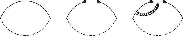
Figure 6. The typical Feynman diagrams which can be factorized into two colored quark lines for the conventional heavy mesons, where the solid line and dashed line denote the light quark and heavy quark, respectively. |
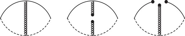
Figure 7. The typical Feynman diagrams which cannot be factorized into two colored quark lines for the conventional heavy mesons, where the solid line and dashed line denote the light quark and heavy quark, respectively. |
where the thresholds ${{\rm{\Delta }}}^{2}=4{m}_{c}^{2}$ and $9{m}_{c}^{2}$ for the QCD spectral densities ${\rho }_{T,\mathrm{QCD}}(s)$ and ${\rho }_{H,\mathrm{QCD}}(s)$, respectively.
3. Numerical results and discussions
where $t=\mathrm{log}\tfrac{{\mu }^{2}}{{{\rm{\Lambda }}}^{2}}$, ${b}_{0}=\tfrac{33-2{n}_{f}}{12\pi }$, ${b}_{1}=\tfrac{153-19{n}_{f}}{24{\pi }^{2}}$, ${b}_{2}\,=\tfrac{2857-\tfrac{5033}{9}{n}_{f}+\tfrac{325}{27}{n}_{f}^{2}}{128{\pi }^{3}}$, ${\rm{\Lambda }}=210\,\mathrm{MeV}$, $292\,\mathrm{MeV}$ and $332\,\mathrm{MeV}$ for the flavors nf = 5, 4 and 3, respectively [37, 38], and evolve all the input parameters to the pertinent energy scales $\mu$ to extract the masses of the scalar ${D}^{* }{\bar{D}}^{* }$, ${D}^{* }{D}^{* }$ tetraquark molecular states and the vector ${D}^{* }{D}^{* }{\bar{D}}^{* }$, ${D}^{* }{D}^{* }{D}^{* }$ hexaquark molecular states with the flavor nf = 4, as we cannot obtain energy scale independent QCD sum rules.
through dispersion relation at the QCD side, and they are scale independent or independent on the energy scale we choose to carry out the operator product expansion
which does not mean
due to the two features inherited from the QCD sum rules:
| • | Perturbative corrections are neglected, even in the QCD sum rules for the traditional mesons, we cannot take into account the perturbative corrections up to arbitrary orders; the higher dimensional vacuum condensates are factorized into lower dimensional ones based on the vacuum saturation, therefore the energy scale dependence of the higher dimensional vacuum condensates is modified. |
| • | Truncations s0 set in, the correlation between the threshold $4/9{m}_{c}^{2}(\mu )$ and continuum threshold s0 is unknown. After performing the Borel transform, we obtain the integrals $\begin{eqnarray}{\int }_{4/9{m}_{c}^{2}(\mu )}^{{s}_{0}}{\rm{d}}{s}{\rho }_{\mathrm{QCD}}(s,\mu )\exp \left(-\displaystyle \frac{s}{{T}^{2}}\right),\end{eqnarray}$ which are sensitive to the c-quark mass ${m}_{c}(\mu )$ or the energy scale $\mu$. Variations of the energy scale $\mu$ can lead to changes of integral ranges $4/9{m}_{c}^{2}(\mu )-{s}_{0}$ of the variable ds besides the QCD spectral densities ${\rho }_{\mathrm{QCD}}(s,\mu )$, therefore changes of the Borel windows and predicted masses and pole residues. |
for the tetraquark molecular states and hexaquark molecular states, respectively [8, 13, 24, 31-35]. Analysis of the $J/\psi $ and ϒ with the famous Cornell potential or Coulomb-potential-plus-linear-potential leads to the constituent quark masses ${m}_{c}=1.84\,\mathrm{GeV}$ and ${m}_{b}=5.17\,\mathrm{GeV}$ [39], we can set the effective c-quark mass equal to the constituent quark mass ${{\mathbb{M}}}_{c}={m}_{c}=1.84\,\mathrm{GeV}$. The old value ${{\mathbb{M}}}_{c}=1.84\,\mathrm{GeV}$ and updated value ${{\mathbb{M}}}_{c}=1.85\,\mathrm{GeV}$ fitted in the QCD sum rules for the hidden-charm tetraquark molecular states are all consistent with the constituent quark mass ${m}_{c}=1.84\,\mathrm{GeV}$ [8, 40]. We can choose the value ${{\mathbb{M}}}_{c}=1.84\pm 0.01\,\mathrm{GeV}$ [13], take the energy scale formula $\mu =\sqrt{{M}_{T}^{2}-{(2{{\mathbb{M}}}_{c})}^{2}}$ and $\sqrt{{M}_{H}^{2}-{(3{{\mathbb{M}}}_{c})}^{2}}$ to improve the convergence of the operator product expansion and enhance the pole contributions. It is a remarkable advantage of the present work.
where the Constants have the values $4{{\mathbb{M}}}_{c}^{2}$ or $9{{\mathbb{M}}}_{c}^{2}$. As we cannot obtain energy scale independent QCD sum rules, we conjecture that the predicted multiquark masses and the pertinent energy scales of the QCD spectral densities have a Regge-trajectory-like relation, see equation (
and define the contributions of the vacuum condensates of dimension n,
where the ${\rho }_{\mathrm{QCD};n}(s)$ are the QCD spectral densities containing the vacuum condensates of dimension n. For the hexaquark (molecular) states, the largest power ${\rho }_{H,\mathrm{QCD}}(s)\propto {s}^{7}$, while for the tetraquark (molecular) states, the largest power ${\rho }_{T,\mathrm{QCD}}(s)\propto {s}^{4}$, it is very difficult to satisfy the two basic criteria of the QCD sum rules simultaneously, we have to resort to some methods to improve the convergent behaviors of the operator product expansion and enhance the pole contributions, the energy scale formula does the work.
Table 1. The Borel parameters, continuum threshold parameters, energy scales of the QCD spectral densities and pole contributions for the ${D}^{* }{\bar{D}}^{* }$, ${D}^{* }{D}^{* }$, ${D}^{* }{D}^{* }{\bar{D}}^{* }$ and ${D}^{* }{D}^{* }{D}^{* }$ tetraquark and hexaquark molecular states. |
| JP | ${T}^{2}({\mathrm{GeV}}^{2})$ | $\sqrt{{s}_{0}}(\mathrm{GeV})$ | $\mu (\mathrm{GeV})$ | Pole |
| ${0}^{+}({D}^{* }{\bar{D}}^{* })$ | 2.8-3.2 | 4.55 ± 0.10 | 1.5 | (41-64)% |
| ${0}^{+}({D}^{* }{D}^{* })$ | 3.0-3.4 | 4.65 ± 0.10 | 1.8 | (41-62)% |
| ${1}^{-}({D}^{* }{D}^{* }{\bar{D}}^{* })$ | 3.9-4.3 | 6.60 ± 0.10 | 2.4 | (41-60)% |
| ${1}^{-}({D}^{* }{D}^{* }{D}^{* })$ | 3.9-4.3 | 6.60 ± 0.10 | 2.4 | (39-60)% |
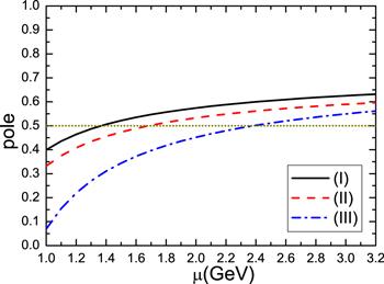
Figure 8. The pole contributions with variations of the energy scales $\mu$ of the QCD spectral densities, where the (I), (II) and (III) correspond to the currents ${J}_{c\bar{c}}(x)$, Jcc(x) and ${J}_{\mu }^{{cc}\bar{c}}(x)$, respectively. The central values of the other parameters are chosen. |

Figure 9. The absolute values of the contributions of the vacuum condensates, where the (I), (II), (III) and (IV) correspond to the currents ${J}_{c\bar{c}}(x)$, Jcc(x), ${J}_{\mu }^{{cc}\bar{c}}(x)$ and ${J}_{\mu }^{{ccc}}(x)$, respectively. The central values of the other parameters are chosen. |
If we set ${{\mathbb{M}}}_{c}={m}_{c}=1.84\,\mathrm{GeV}$, we can obtain the dash-dotted lines ${M}_{T}=\sqrt{{\mu }^{2}+4\times {(1.84\mathrm{GeV})}^{2}}$ and ${M}_{H}=\sqrt{{\mu }^{2}+9\times {(1.84\mathrm{GeV})}^{2}}$ in figure 10, which intersect with the lines of the masses of the ${D}^{* }{\bar{D}}^{* }$, ${D}^{* }{D}^{* }$ and ${D}^{* }{D}^{* }{\bar{D}}^{* }$ tetraquark or hexaquark molecular states at the energy scales about $\mu =1.5\,\mathrm{GeV}$, $1.8\,\mathrm{GeV}$ and $2.4\,\mathrm{GeV}$, respectively. In this way, we choose the energy scales of the QCD spectral densities in a consistent way.
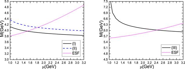
Figure 10. The masses of the tetraquark and hexaquark molecular states with variations of the energy scales $\mu$ of the QCD spectral densities, where the (I), (II) and (III) correspond to the ${D}^{* }{\bar{D}}^{* }$, ${D}^{* }{D}^{* }$ and ${D}^{* }{D}^{* }{\bar{D}}^{* }$ tetraquark and hexaquark molecular states, respectively, the ESF denotes the formulas $M=\sqrt{{\mu }^{2}+4\times {(1.84\mathrm{GeV})}^{2}}$ and $\sqrt{{\mu }^{2}+9\times {(1.84\mathrm{GeV})}^{2}}$, respectively. |
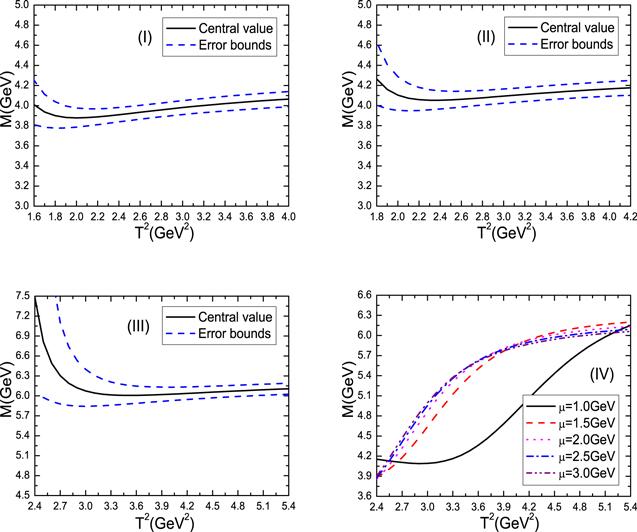
Figure 11. The masses of the tetraquark and hexaquark molecular states with variations of the Borel parameters T2, where the (I), (II), (III) and (IV) correspond to the ${D}^{* }{\bar{D}}^{* }$, ${D}^{* }{D}^{* }$, ${D}^{* }{D}^{* }{\bar{D}}^{* }$ and ${D}^{* }{D}^{* }{D}^{* }$ tetraquark and hexaquark molecular states, respectively. |
Table 2. The masses and pole residues for the ${D}^{* }{\bar{D}}^{* }$, ${D}^{* }{D}^{* }$ and ${D}^{* }{D}^{* }{\bar{D}}^{* }$ tetraquark and hexaquark molecular states. |
| JP | ${M}_{T/H}$ | ${\lambda }_{T/H}$ |
| ${0}^{+}({D}^{* }{\bar{D}}^{* })$ | $3.98\pm 0.09\,\mathrm{GeV}$ | $(4.05\pm 0.70)\times {10}^{-2}{\mathrm{GeV}}^{5}$ |
| ${0}^{+}({D}^{* }{D}^{* })$ | $4.11\pm 0.09\,\mathrm{GeV}$ | $(8.36\pm 1.32)\times {10}^{-2}{\mathrm{GeV}}^{5}$ |
| ${1}^{-}({D}^{* }{D}^{* }{\bar{D}}^{* })$ | $6.03\pm 0.11\,\mathrm{GeV}$ | $(3.14\pm 0.55)\times {10}^{-3}{\mathrm{GeV}}^{8}$ |
where the ${\varepsilon }_{\alpha }$ is the polarization vector of the D* meson. The renormalized self-energies due to the intermediate meson-loops contribute a finite imaginary part to modify the dispersion relation,
We take into account the finite width effects by the following simple replacement of the hadronic spectral densities,
then the hadron sides of the QCD sum rules in equations (
where the ${{\rm{\Delta }}}^{2}$ are the two-meson or three-meson thresholds. The net effects of the intermediate meson-loops can be absorbed into the pole residues ${\tilde{\lambda }}_{T/H}$ safely without affecting the predicted tetraquark and hexaquark molecule masses. Even for the ${Z}_{c}(4200)$, the width is as large as ${370}_{-70}^{+70}{}_{-132}^{+70}\,\mathrm{MeV}$, the finite width effects can be safely absorbed into the pole residues [43], so the zero width approximation in the hadronic spectral density works very well.
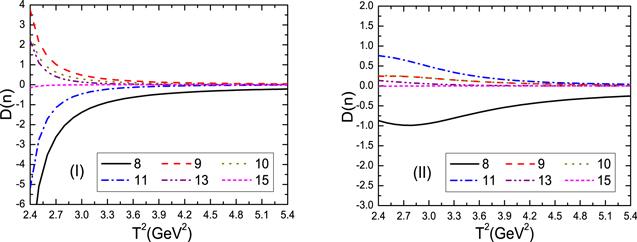
Figure 12. The contributions of the higher dimensional vacuum condensates with variations of the Borel parameters T2 for the central values of other parameters, where the (I) and (II) correspond to the currents ${J}_{\mu }^{{cc}\bar{c}}(x)$ and ${J}_{\mu }^{{ccc}}(x)$, respectively. |
4. Conclusion
Appendix
$\begin{eqnarray}\begin{array}{l}{\rho }_{T}^{c\bar{c}}(s,\mu )=\displaystyle \frac{3}{512{\pi }^{6}}\displaystyle \int {\rm{d}}{y}{\rm{d}}{z}\,{yz}{\left(1-y-z\right)}^{2}\\ \ \ \times \,{\left(s-{\overline{m}}_{c}^{2}\right)}^{3}\left(3s-{\overline{m}}_{c}^{2}\right)\\ \ \ -\,\displaystyle \frac{3{m}_{c}\langle \bar{q}q\rangle }{16{\pi }^{4}}\displaystyle \int {\rm{d}}{y}{\rm{d}}{z}\,y\left(1-y-z\right)\left(s-{\overline{m}}_{c}^{2}\right)\left(2s-{\overline{m}}_{c}^{2}\right)\\ \ \ +\,\displaystyle \frac{{m}_{c}\langle \bar{q}{g}_{s}\sigma {Gq}\rangle }{64{\pi }^{4}}\displaystyle \int {\rm{d}}{y}{\rm{d}}{z}\,y\left(7s-6{\overline{m}}_{c}^{2}\right)+\displaystyle \frac{{m}_{c}^{2}\langle \bar{q}q{\rangle }^{2}}{4{\pi }^{2}}\displaystyle \int {\rm{d}}{y}\,\\ \ \ -\,\displaystyle \frac{{m}_{c}^{2}\langle \bar{q}q\rangle \langle \bar{q}{g}_{s}\sigma {Gq}\rangle }{8{\pi }^{2}}\displaystyle \int {\rm{d}}{y}\left(1+\displaystyle \frac{s}{{T}^{2}}\right)\delta \left(s-{\widetilde{m}}_{c}^{2}\right)\\ \ \ +\,\displaystyle \frac{{m}_{c}^{2}\langle \bar{q}{g}_{s}\sigma {Gq}{\rangle }^{2}}{64{\pi }^{2}{T}^{6}}\displaystyle \int {\rm{d}}{y}\,{s}^{2}\delta \left(s-{\widetilde{m}}_{c}^{2}\right)\\ \ \ -\,\displaystyle \frac{{m}_{c}^{2}}{128{\pi }^{4}}\left\langle \displaystyle \frac{{\alpha }_{s}{GG}}{\pi }\right\rangle \displaystyle \int {\rm{d}}{y}{\rm{d}}{z}\,\displaystyle \frac{z{\left(1-y-z\right)}^{2}}{{y}^{2}}\left(3s-2{\overline{m}}_{c}^{2}\right)\\ \ \ +\,\displaystyle \frac{{m}_{c}^{3}\langle \bar{q}q\rangle }{96{\pi }^{2}}\left\langle \displaystyle \frac{{\alpha }_{s}{GG}}{\pi }\right\rangle \displaystyle \int {\rm{d}}{y}{\rm{d}}{z}\left(1+\displaystyle \frac{z}{y}\right)\\ \ \ \times \,\displaystyle \frac{(1-y-z)}{{y}^{2}}\left(1+\displaystyle \frac{s}{{T}^{2}}\right)\delta \left(s-{\overline{m}}_{c}^{2}\right)\\ \ \ +\,\displaystyle \frac{{m}_{c}\langle \bar{q}q\rangle }{32{\pi }^{2}}\left\langle \displaystyle \frac{{\alpha }_{s}{GG}}{\pi }\right\rangle \displaystyle \int {\rm{d}}{y}{\rm{d}}{z}\left[1-\displaystyle \frac{z(1-y-z)}{{y}^{2}}\right]\end{array}\end{eqnarray}$
$\begin{eqnarray}\begin{array}{l}\times \,\left[2+s\,\delta \left(s-{\overline{m}}_{c}^{2}\right)\right]\\ \ \ -\,\displaystyle \frac{{m}_{c}^{4}\langle \bar{q}q{\rangle }^{2}}{36{T}^{4}}\left\langle \displaystyle \frac{{\alpha }_{s}{GG}}{\pi }\right\rangle \displaystyle \int {\rm{d}}{y}\,\displaystyle \frac{1}{{y}^{3}}\delta \left(s-{\widetilde{m}}_{c}^{2}\right)\\ \ \ +\,\displaystyle \frac{{m}_{c}^{2}\langle \bar{q}q{\rangle }^{2}}{72{T}^{6}}\displaystyle \int {\rm{d}}{y}\,{s}^{2}\delta \left(s-{\widetilde{m}}_{c}^{2}\right)\\ \ \ +\,\displaystyle \frac{{m}_{c}^{2}\langle \bar{q}q{\rangle }^{2}}{12{T}^{2}}\left\langle \displaystyle \frac{{\alpha }_{s}{GG}}{\pi }\right\rangle \displaystyle \int {\rm{d}}{y}\,\displaystyle \frac{1}{{y}^{2}}\delta \left(s-{\widetilde{m}}_{c}^{2}\right)\\ \ \ +\,\displaystyle \frac{\langle \bar{q}{g}_{s}\sigma {Gq}{\rangle }^{2}}{256{\pi }^{2}{T}^{2}}\displaystyle \int {\rm{d}}{y}\,s\delta \left(s-{\widetilde{m}}_{c}^{2}\right)\\ \ \ -\,\displaystyle \frac{{m}_{c}\langle \bar{q}q\rangle }{192{\pi }^{2}}\left\langle \displaystyle \frac{{\alpha }_{s}{GG}}{\pi }\right\rangle \displaystyle \int {\rm{d}}{y}\,y\left[2+s\delta \left(s-{\widetilde{m}}_{c}^{2}\right)\right],\end{array}\end{eqnarray}$
$\begin{eqnarray*}\begin{array}{l}{\rho }_{T}^{{cc}}(s,\mu )=\displaystyle \frac{7}{512{\pi }^{6}}\displaystyle \int {\rm{d}}{y}{\rm{d}}{z}\,{yz}{\left(1-y-z\right)}^{2}\\ \ \ \times \,{\left(s-{\overline{m}}_{c}^{2}\right)}^{3}\left(3s-{\overline{m}}_{c}^{2}\right)\\ \ \ -\,\displaystyle \frac{{m}_{c}^{2}}{512{\pi }^{6}}\displaystyle \int {\rm{d}}{y}{\rm{d}}{z}{\left(1-y-z\right)}^{2}{\left(s-{\overline{m}}_{c}^{2}\right)}^{3}\\ \ \ -\,\displaystyle \frac{{m}_{c}\langle \bar{q}q\rangle }{2{\pi }^{4}}\displaystyle \int {\rm{d}}{y}{\rm{d}}{z}\,y\left(1-y-z\right)\left(s-{\overline{m}}_{c}^{2}\right)\left(2s-{\overline{m}}_{c}^{2}\right)\\ \ \ +\,\displaystyle \frac{{m}_{c}\langle \bar{q}{g}_{s}\sigma {Gq}\rangle }{8{\pi }^{4}}\displaystyle \int {\rm{d}}{y}{\rm{d}}{z}\,y\left(3s-2{\overline{m}}_{c}^{2}\right)\\ \ \ -\,\displaystyle \frac{\langle \bar{q}q{\rangle }^{2}}{24{\pi }^{2}}\displaystyle \int {\rm{d}}{y}\,y(1-y)\left(3s-2{\widetilde{m}}_{c}^{2}\right)\\ \ \ +\,\displaystyle \frac{7{m}_{c}^{2}\langle \bar{q}q{\rangle }^{2}}{12{\pi }^{2}}\displaystyle \int {\rm{d}}{y}\,\\ \ \ +\,\displaystyle \frac{\langle \bar{q}q\rangle \langle \bar{q}{g}_{s}\sigma {Gq}\rangle }{48{\pi }^{2}}\displaystyle \int {\rm{d}}{y}\,y(1-y)\\ \ \ \times \,\left[6+\left(4s+\displaystyle \frac{{s}^{2}}{{T}^{2}}\right)\delta \left(s-{\widetilde{m}}_{c}^{2}\right)\right]\\ \ \ -\,\displaystyle \frac{7{m}_{c}^{2}\langle \bar{q}q\rangle \langle \bar{q}{g}_{s}\sigma {Gq}\rangle }{24{\pi }^{2}}\displaystyle \int {\rm{d}}{y}\left(1+\displaystyle \frac{s}{{T}^{2}}\right)\delta \left(s-{\widetilde{m}}_{c}^{2}\right)\\ \ \ -\,\displaystyle \frac{\langle \bar{q}{g}_{s}\sigma {Gq}{\rangle }^{2}}{384{\pi }^{2}}\displaystyle \int {\rm{d}}{y}\,y(1-y)\\ \ \ \times \,\left(6+\displaystyle \frac{6s}{{T}^{2}}+\displaystyle \frac{3{s}^{2}}{{T}^{4}}+\displaystyle \frac{{s}^{3}}{{T}^{6}}\right)\delta (s-{\widetilde{m}}_{c}^{2})\\ \ \ +\,\displaystyle \frac{7{m}_{c}^{2}\langle \bar{q}{g}_{s}\sigma {Gq}{\rangle }^{2}}{192{\pi }^{2}{T}^{6}}\displaystyle \int {\rm{d}}{y}\,{s}^{2}\delta \left(s-{\widetilde{m}}_{c}^{2}\right)\\ \ \ -\displaystyle \frac{7{m}_{c}^{2}}{384{\pi }^{4}}\left\langle \displaystyle \frac{{\alpha }_{s}{GG}}{\pi }\right\rangle \displaystyle \int {\rm{d}}{y}{\rm{d}}{z}\,\displaystyle \frac{z{\left(1-y-z\right)}^{2}}{{y}^{2}}\left(3s-2{\overline{m}}_{c}^{2}\right)\\ \ \ +\,\displaystyle \frac{{m}_{c}^{4}}{768{\pi }^{4}}\left\langle \displaystyle \frac{{\alpha }_{s}{GG}}{\pi }\right\rangle \displaystyle \int {\rm{d}}{y}{\rm{d}}{z}\,\displaystyle \frac{{\left(1-y-z\right)}^{2}}{{y}^{3}}\\ \ \ +\displaystyle \frac{{m}_{c}^{3}\langle \bar{q}q\rangle }{36{\pi }^{2}}\left\langle \displaystyle \frac{{\alpha }_{s}{GG}}{\pi }\right\rangle \displaystyle \int {\rm{d}}{y}{\rm{d}}{z}\left(1+\displaystyle \frac{z}{y}\right)\\ \ \ \times \,\displaystyle \frac{1-y-z}{{y}^{2}}\left(1+\displaystyle \frac{s}{{T}^{2}}\right)\delta (s-{\overline{m}}_{c}^{2})\\ \ \ +\,\displaystyle \frac{{m}_{c}^{2}\langle \bar{q}q{\rangle }^{2}}{216{T}^{4}}\left\langle \displaystyle \frac{{\alpha }_{s}{GG}}{\pi }\right\rangle \displaystyle \int {\rm{d}}{y}\,\displaystyle \frac{1-y}{{y}^{2}}s\,\delta \left(s-{\widetilde{m}}_{c}^{2}\right)\\ \ \ -\,\displaystyle \frac{7{m}_{c}^{4}\langle \bar{q}q{\rangle }^{2}}{108{T}^{4}}\left\langle \displaystyle \frac{{\alpha }_{s}{GG}}{\pi }\right\rangle \displaystyle \int {\rm{d}}{y}\,\displaystyle \frac{1}{{y}^{3}}\delta \left(s-{\widetilde{m}}_{c}^{2}\right)\\ \ \ -\displaystyle \frac{{m}_{c}^{2}}{256{\pi }^{4}}\left\langle \displaystyle \frac{{\alpha }_{s}{GG}}{\pi }\right\rangle \displaystyle \int {\rm{d}}{y}{\rm{d}}{z}\,\displaystyle \frac{{\left(1-y-z\right)}^{2}}{{y}^{2}}\left(s-{\overline{m}}_{c}^{2}\right)\\ \ \ +\,\displaystyle \frac{{m}_{c}\langle \bar{q}q\rangle }{48{\pi }^{2}}\left\langle \displaystyle \frac{{\alpha }_{s}{GG}}{\pi }\right\rangle \displaystyle \int {\rm{d}}{y}{\rm{d}}{z}\\ \ \ \times \,\left[4-\displaystyle \frac{4z(1-y-z)}{{y}^{2}}+\displaystyle \frac{1-y-z}{z}-\displaystyle \frac{z}{y}\right]\\ \ \ \times \,\left[2+s\delta \left(s-{\overline{m}}_{c}^{2}\right)\right]\end{array}\end{eqnarray*}$
$\begin{eqnarray*}\begin{array}{l}\ \ +\displaystyle \frac{7{m}_{c}^{2}\langle \bar{q}q{\rangle }^{2}}{36{T}^{2}}\left\langle \displaystyle \frac{{\alpha }_{s}{GG}}{\pi }\right\rangle \displaystyle \int {\rm{d}}{y}\,\displaystyle \frac{1}{{y}^{2}}\delta \left(s-{\widetilde{m}}_{c}^{2}\right)\\ \ \ -\,\displaystyle \frac{1}{128{\pi }^{4}}\left\langle \displaystyle \frac{{\alpha }_{s}{GG}}{\pi }\right\rangle \displaystyle \int {\rm{d}}{y}{\rm{d}}{z}\,{yz}\left(s-{\overline{m}}_{c}^{2}\right)\left(2s-{\overline{m}}_{c}^{2}\right)\\ \ \ -\,\displaystyle \frac{{m}_{c}^{2}}{256{\pi }^{4}}\left\langle \displaystyle \frac{{\alpha }_{s}{GG}}{\pi }\right\rangle \displaystyle \int {\rm{d}}{y}{\rm{d}}{z}\,\displaystyle \frac{4-3y-4z}{y}\left(s-{\overline{m}}_{c}^{2}\right)\\ \ \ -\,\displaystyle \frac{1}{256{\pi }^{4}}\left\langle \displaystyle \frac{{\alpha }_{s}{GG}}{\pi }\right\rangle \displaystyle \int {\rm{d}}{y}{\rm{d}}{z}{\left(1-y-z\right)}^{2}\\ \ \ \times \,\left(s-{\overline{m}}_{c}^{2}\right)\left(2s-{\overline{m}}_{c}^{2}\right)\\ \ \ -\,\displaystyle \frac{\langle \bar{q}q{\rangle }^{2}}{144}\left\langle \displaystyle \frac{{\alpha }_{s}{GG}}{\pi }\right\rangle \displaystyle \int {\rm{d}}{y}\left(1+\displaystyle \frac{5s}{{T}^{2}}\right)\delta \left(s-{\widetilde{m}}_{c}^{2}\right)\\ \ \ -\,\displaystyle \frac{{m}_{c}\langle \bar{q}{g}_{s}\sigma {Gq}\rangle }{32{\pi }^{4}}\displaystyle \int {\rm{d}}{y}{\rm{d}}{z}\left(1-2y-z\right)\left(3s-2{\overline{m}}_{c}^{2}\right)\end{array}\end{eqnarray*}$
$\begin{eqnarray}\begin{array}{l}-\displaystyle \frac{\langle \bar{q}q\rangle \langle \bar{q}{g}_{s}\sigma {Gq}\rangle }{24{\pi }^{2}}\displaystyle \int {\rm{d}}{y}\left(1-y\right)\left[2+s\,\delta \left(s-{\widetilde{m}}_{c}^{2}\right)\right]\\ \ \ +\,\displaystyle \frac{\langle \bar{q}{g}_{s}\sigma {Gq}{\rangle }^{2}}{96{\pi }^{2}}\displaystyle \int {\rm{d}}{y}\left(1-y\right)\left(2+\displaystyle \frac{2s}{{T}^{2}}+\displaystyle \frac{{s}^{2}}{{T}^{4}}\right)\delta \left(s-{\widetilde{m}}_{c}^{2}\right)\\ \ \ -\,\displaystyle \frac{\langle \bar{q}{g}_{s}\sigma {Gq}{\rangle }^{2}}{192{\pi }^{2}}\displaystyle \int {\rm{d}}{y}\left(1+\displaystyle \frac{s}{{T}^{2}}\right)\delta \left(s-{\widetilde{m}}_{c}^{2}\right)\\ \ \ +\,\displaystyle \frac{\langle \bar{q}{g}_{s}\sigma {Gq}{\rangle }^{2}}{128{\pi }^{2}{T}^{2}}\displaystyle \int {\rm{d}}{y}\,s\,\delta \left(s-{\widetilde{m}}_{c}^{2}\right)\\ \ \ -\displaystyle \frac{{m}_{c}\langle \bar{q}q\rangle }{72{\pi }^{2}}\left\langle \displaystyle \frac{{\alpha }_{s}{GG}}{\pi }\right\rangle \displaystyle \int {\rm{d}}{y}\,y\left[2+s\,\delta \left(s-{\widetilde{m}}_{c}^{2}\right)\right]\\ \ \ -\,\displaystyle \frac{\langle \bar{q}q{\rangle }^{2}}{432}\left\langle \displaystyle \frac{{\alpha }_{s}{GG}}{\pi }\right\rangle \displaystyle \int {\rm{d}}{y}\,y(1-y)\\ \ \ \times \,\left(6+\displaystyle \frac{6s}{{T}^{2}}+\displaystyle \frac{3{s}^{2}}{{T}^{4}}+\displaystyle \frac{{s}^{3}}{{T}^{6}}\right)\delta \left(s-{\widetilde{m}}_{c}^{2}\right)\\ \ \ +\,\displaystyle \frac{7{m}_{c}^{2}\langle \bar{q}q{\rangle }^{2}}{216{T}^{6}}\left\langle \displaystyle \frac{{\alpha }_{s}{GG}}{\pi }\right\rangle \displaystyle \int {\rm{d}}{y}\,{s}^{2}\delta \left(s-{\widetilde{m}}_{c}^{2}\right),\end{array}\end{eqnarray}$