


1. Introduction
2. MEMF in Dimension 1
If a real function f is Cn on $[a,b]$ for some $n\in {{\mathbb{N}}}^{+}$ and a, $b\in {\mathbb{Z}}$ with $a\lt b$, then for given $m,p\in {\mathbb{N}}$ with $m\leqslant b-a$, the summation of f over integer points on $[a,b]$ can be evaluated by the formula
Two modifications are made to the original Euler–Maclaurin formula. (i) We sum over the first m terms explicitly, which is trival but necessary for some quantum systems at low temperature. (ii) We keep part of the original remainder in our calculations to improve the accuracy of the summation.
We apply the Euler–Maclaurin formula to the summation on the left hand side after modification (i) and obtain
If the conditions in theorem
We reveal the following connections to the Euler–Maclaurin formula and to the Poisson summation formula.
| 1.Taking $m=0,p=0$ in theorem | |
| 2.Taking $m=0,n=1$ in theorem $\begin{eqnarray*}\displaystyle \sum _{i=a}^{b}f(i)=\displaystyle \sum _{k=-\infty }^{+\infty }{\int }_{a}^{b}f(x){{\rm{e}}}^{{\rm{i}}2\pi {kx}}{\rm{d}}x+\displaystyle \frac{f(a)+f(b)}{2}.\end{eqnarray*}$ Furthermore, if all the terms in the above equation are finite and the summation on the left hand side converges as $a\to -\infty $ and $b\to +\infty $, then it becomes the Poisson summation formula $\begin{eqnarray*}\displaystyle \sum _{i=-\infty }^{+\infty }f(i)=\displaystyle \sum _{k=-\infty }^{+\infty }{\int }_{-\infty }^{+\infty }f(x){{\rm{e}}}^{{\rm{i}}2\pi {kx}}{\rm{d}}x.\end{eqnarray*}$ |
If the conditions in theorem
| 1. $\begin{eqnarray*}| {R}_{{mnp}}| \leqslant {R}_{{mnp}}^{A}\equiv {T}_{n,p}{\int }_{a^{\prime} }^{b}\left|{f}^{(n)}(x)\right|{\rm{d}}x.\end{eqnarray*}$ | |
| 2.If n is odd, and ${f}^{(n)}(x)$ is monotone with respect to x on $[a^{\prime} ,b]$, then $\begin{eqnarray*}\left|{R}_{{mnp}}\right|\leqslant {R}_{{mnp}}^{B}\equiv 2{T}_{n+1,p}\left|{M}_{n}(a^{\prime} ,b)\right|.\end{eqnarray*}$ If n is even, and ${f}^{(n)}(x)$ is monotone with respect to x on $[a^{\prime} ,b]$, then $\begin{eqnarray*}\left|{R}_{{mnp}}\right|\leqslant {R}_{{mnp}}^{C}\equiv {T}_{n+1,p}\left|{M}_{n}(a^{\prime} ,b)\right|.\end{eqnarray*}$ |
| 1.Compute $\begin{eqnarray*}\begin{array}{l}\left|{R}_{{mnp}}\right|=\left|{\left(-1\right)}^{n}{\displaystyle \int }_{a^{\prime} }^{b}\displaystyle \sum _{| k| \gt p}\displaystyle \frac{{{\rm{e}}}^{{\rm{i}}2\pi {kx}}}{{\left({\rm{i}}2\pi k\right)}^{n}}{f}^{(n)}(x){\rm{d}}x\right|\leqslant {\displaystyle \int }_{a^{\prime} }^{b}\displaystyle \sum _{| k| \gt p}\left|\displaystyle \frac{{{\rm{e}}}^{{\rm{i}}2\pi {kx}}}{{\left({\rm{i}}2\pi k\right)}^{n}}{f}^{(n)}(x)\right|{\rm{d}}x\\ \qquad \quad={T}_{n,p}{\displaystyle \int }_{a^{\prime} }^{b}\left|{f}^{(n)}(x)\right|{\rm{d}}x.\end{array}\end{eqnarray*}$ | |
| 2.For odd n, we estimate $\begin{eqnarray*}\begin{array}{l}\left|{R}_{{mnp}}\right|=\left|{\left(-1\right)}^{n}{\displaystyle \int }_{a^{\prime} }^{b}\displaystyle \sum _{| k| \gt p}\displaystyle \frac{{{\rm{e}}}^{{\rm{i}}2\pi {kx}}}{{\left({\rm{i}}2\pi k\right)}^{n}}{f}^{(n)}(x){\rm{d}}x\right|\\ \quad \leqslant \displaystyle \frac{1}{{\left(2\pi \right)}^{n}}\displaystyle \sum _{k\gt p}\displaystyle \frac{2}{{k}^{n}}\left|{\displaystyle \int }_{a^{\prime} }^{b}\sin (2\pi {kx}){f}^{(n)}(x){\rm{d}}x\right|\\ =\ \displaystyle \frac{1}{{\left(2\pi \right)}^{n}}\displaystyle \sum _{k\gt p}\displaystyle \frac{2}{{k}^{n}}\ \left|\displaystyle \sum _{j=1}^{2k(b-a^{\prime} )}{\displaystyle \int }_{a^{\prime} +\tfrac{j-1}{2k}}^{a^{\prime} +\tfrac{j}{2k}}\sin (2\pi {kx})\left({f}^{(n)}(x)-{f}^{(n)}(b)\right){\rm{d}}x\right|.\end{array}\end{eqnarray*}$ Note that the summation is an alternating summation, we have $\begin{eqnarray*}\begin{array}{l}\left|{R}_{{mnp}}\right|\leqslant \displaystyle \frac{1}{{\left(2\pi \right)}^{n}}\displaystyle \sum _{k\gt p}\displaystyle \frac{2}{{k}^{n}}\left|{\displaystyle \int }_{a^{\prime} }^{a^{\prime} +\tfrac{1}{2k}}\sin (2\pi {kx})\left({f}^{(n)}(x)-{f}^{(n)}(b)\right){\rm{d}}x\right|\\ \,\leqslant \,\displaystyle \frac{1}{{\left(2\pi \right)}^{n}}\displaystyle \sum _{k\gt p}\displaystyle \frac{2}{{k}^{n}}\left|{f}^{(n)}(a^{\prime} )-{f}^{(n)}(b)\right|\displaystyle \frac{1}{\pi k}\\ \,=\ 2{T}_{n+1,p}\left|{M}_{n}(a^{\prime} ,b)\right|.\end{array}\end{eqnarray*}$ Similarly, for even n, we estimate $\begin{eqnarray*}\begin{array}{l}\left|{R}_{{mnp}}\right|=\left|{\left(-1\right)}^{n}{\displaystyle \int }_{a^{\prime} }^{b}\displaystyle \sum _{| k| \gt p}\displaystyle \frac{{{\rm{e}}}^{{\rm{i}}2\pi {kx}}}{{\left({\rm{i}}2\pi k\right)}^{n}}{f}^{(n)}(x){\rm{d}}x\right|\\ \,\leqslant \,\displaystyle \frac{1}{{\left(2\pi \right)}^{n}}\displaystyle \sum _{k\gt p}\displaystyle \frac{2}{{k}^{n}}\left|{\displaystyle \int }_{a^{\prime} }^{b}\cos (2\pi {kx}){f}^{(n)}(x){\rm{d}}x\right|\\ \,=\ \displaystyle \frac{1}{{\left(2\pi \right)}^{n}}\displaystyle \sum _{k\gt p}\displaystyle \frac{2}{{k}^{n}}\left|\left({\displaystyle \int }_{a^{\prime} }^{a^{\prime} +\tfrac{1}{4k}}+\displaystyle \sum _{j=1}^{2k(b-a^{\prime} )-1}{\displaystyle \int }_{a^{\prime} +\tfrac{j-1/2}{2k}}^{a^{\prime} +\tfrac{j+1/2}{2k}}+{\displaystyle \int }_{b-\tfrac{1}{4k}}^{b}\right)\\ \times \cos (2\pi {kx})\left({f}^{(n)}(x)-{f}^{(n)}(b)\right){\rm{d}}x\right|\\ \,\leqslant \,\displaystyle \frac{1}{{\left(2\pi \right)}^{n}}\displaystyle \sum _{k\gt p}\displaystyle \frac{2}{{k}^{n}}{\displaystyle \int }_{a^{\prime} }^{a^{\prime} +\tfrac{1}{4k}}\cos (2\pi {kx})\left|{f}^{(n)}(x)-{f}^{(n)}(b)\right|{\rm{d}}x\\ \,\leqslant \,\displaystyle \frac{1}{{\left(2\pi \right)}^{n}}\displaystyle \sum _{k\gt p}\displaystyle \frac{2}{{k}^{n}}\left|{f}^{(n)}(a^{\prime} )-{f}^{(n)}(b)\right|\displaystyle \frac{1}{2\pi k}\\ \,=\,\ {T}_{n+1,p}\left|{M}_{n}(a^{\prime} ,b)\right|.\end{array}\end{eqnarray*}$ |
If the conditions in theorem
3. Generalization to Dimension 2
Let D be the rectangle
We rewrite equation (
Note that (i) equation (
Suppose P is a set of integer pairs with ${P}_{0}\subset P$, ${P}_{1}=P-{P}_{0}$, and
Again, dropping the remainder term R, an approximation of the original summation in Dimension 2 is obtained.
If f satisfies the conditions in theorem
Equation (
Obviously, for given n, $n^{\prime} $ and f, one can always choose proper p and $p^{\prime} $ to achieve as high accuracy as expected. For $n^{\prime} =n$ and $p^{\prime} =p$, the formula is simpler as follows.
$n=n^{\prime} $ and $p=p^{\prime} $. If f satisfies the conditions in theorem
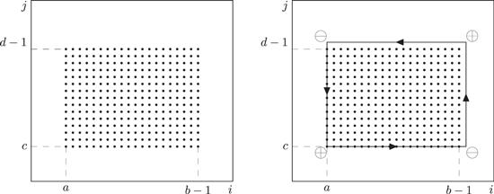
Figure 1. Summation points (left) in lemma |
4. Applications
4.1. Partition function of a one-dimensional infinite square well
4.1.1. Partition function
4.1.2. Remainder estimation
An upper bound of Hermite polynomials can be estimated by
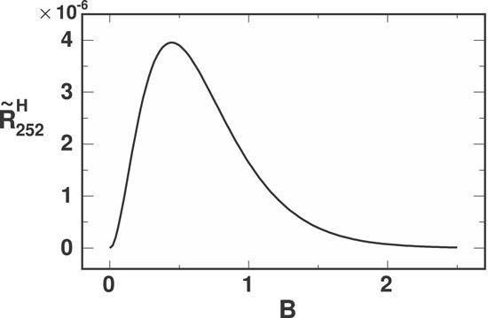
Figure 2. The error bound ${\tilde{R}}_{252}^{H}$ [defined in equation ( |
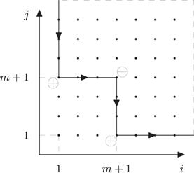
Figure 3. Summation region of the partition function of a two-dimensional square well. |
Table 1. Approximate values of the first several xn and gn(xn). |
| n | 2 | 3 | 4 | 5 | 6 | 7 | 8 | 9 | 10 |
|---|---|---|---|---|---|---|---|---|---|
| xn | 1.534 | 2.052 | 2.476 | 2.843 | 3.170 | 3.467 | 3.742 | 3.999 | 4.240 |
| gn(xn) | 1.374 | 1.584 | 1.772 | 1.942 | 2.099 | 2.245 | 2.382 | 2.512 | 2.635 |
Table 2. Approximate values of ${\bar{R}}_{{np}}^{A}$ [defined in equation ( |
| n | 3 | 5 | 7 | 9 | 11 | 13 | 15 |
|---|---|---|---|---|---|---|---|
| p | |||||||
| 0 | 7.8 × 10⁻² | 1.5 × 10⁻² | 5.0 × 10⁻³ | 2.2 × 10⁻³ | 1.2 × 10⁻³ | 7.8 × 10⁻⁴ | 5.9 × 10⁻⁴ |
| 1 | 1.3 × 10⁻² | 5.4 × 10⁻⁴ | 4.1 × 10⁻⁵ | 4.4 × 10⁻⁶ | 6.0 × 10⁻⁷ | 9.6 × 10⁻⁸ | 1.8 × 10⁻⁸ |
| 2 | 5.0 × 10⁻³ | 8.3 × 10⁻⁵ | 2.7 × 10⁻⁶ | 1.2 × 10⁻⁷ | 7.1 × 10⁻⁹ | 5.0 × 10⁻¹⁰ | 4.2 × 10⁻¹¹ |
| 3 | 2.6 × 10⁻³ | 2.3 × 10⁻⁵ | 3.9 × 10⁻⁷ | 9.8 × 10⁻⁹ | 3.2 × 10⁻¹⁰ | 1.2 × 10⁻¹¹ | 5.7 × 10⁻¹³ |
| 4 | 1.6 × 10⁻³ | 8.6 × 10⁻⁶ | 9.2 × 10⁻⁸ | 1.4 × 10⁻⁹ | 2.9 × 10⁻¹¹ | 7.1 × 10⁻¹³ | 2.1 × 10⁻¹⁴ |
Table 3. Approximate values of ${\tilde{R}}_{0{np}}^{H}$ [defined in equation ( |
| n | 3 | 5 | 7 | 9 | 11 | 13 | 15 |
|---|---|---|---|---|---|---|---|
| p | |||||||
| 0 | 6.5 × 10⁻² | 1.6 × 10⁻² | 6.4 × 10⁻³ | 3.2 × 10⁻³ | 1.9 × 10⁻³ | 1.4 × 10⁻³ | 1.1 × 10⁻³ |
| 1 | 1.1 × 10⁻² | 5.8 × 10⁻⁴ | 5.3 × 10⁻⁵ | 6.4 × 10⁻⁶ | 9.5 × 10⁻⁷ | 1.7 × 10⁻⁷ | 3.4 × 10⁻⁸ |
| 2 | 4.1 × 10⁻³ | 9. × 10−5 | 3.4 × 10⁻⁶ | 1.8 × 10⁻⁷ | 1.1 × 10⁻⁸ | 8.8 × 10⁻¹⁰ | 7.8 × 10⁻¹¹ |
| 3 | 2.2 × 10⁻³ | 2.5 × 10⁻⁵ | 5.0 × 10⁻⁷ | 1.4 × 10⁻⁸ | 5.1 × 10⁻¹⁰ | 2.2 × 10⁻¹¹ | 1.1 × 10⁻¹² |
| 4 | 1.3 × 10⁻³ | 9.3 × 10⁻⁶ | 1.2 × 10⁻⁷ | 2.1 × 10⁻⁹ | 4.6 × 10⁻¹¹ | 1.2 × 10⁻¹² | 3.9 × 10⁻¹⁴ |
4.2. Partition function of a quantum rotator
4.2.1. Partition function
4.2.2. Remainder estimation
4.3. Partition function of a two-dimensional infinite square well
4.3.1. Partition function
4.3.2. Remainder estimation
Table 4. ${\tilde{R}}_{{np},{np}}^{H}$ for square well with B = 1 and m = 0. |
| n | 3 | 5 | 7 | 9 | 11 | 13 | 15 |
|---|---|---|---|---|---|---|---|
| p | |||||||
| 0 | 2.2 × 10⁻² | 4.7 × 10⁻³ | 1.6 × 10⁻³ | 7.2 × 10⁻⁴ | 4.0 × 10⁻⁴ | 2.6 × 10⁻⁴ | 2.0 × 10⁻⁴ |
| 1 | 5.8 × 10⁻³ | 2.6 × 10⁻⁴ | 2.1 × 10⁻⁵ | 2.3 × 10⁻⁶ | 3.1 × 10⁻⁷ | 5.1 × 10⁻⁸ | 9.6 × 10⁻⁹ |
| 2 | 3.2 × 10⁻³ | 5.8 × 10⁻⁵ | 1.9 × 10⁻⁶ | 9.0 × 10⁻⁸ | 5.3 × 10⁻⁹ | 3.8 × 10⁻¹⁰ | 3.2 × 10⁻¹¹ |
| 3 | 2.1 × 10⁻³ | 2.1 × 10⁻⁵ | 3.7 × 10⁻⁷ | 9.5 × 10⁻⁹ | 3.1 × 10⁻¹⁰ | 1.2 × 10⁻¹¹ | 5.7 × 10⁻¹³ |
| 4 | 1.6 × 10⁻³ | 9.7 × 10⁻⁶ | 1.1 × 10⁻⁷ | 1.7 × 10⁻⁹ | 3.5 × 10⁻¹¹ | 8.7 × 10⁻¹³ | 2.6 × 10⁻¹⁴ |