


1. Introduction
2. The model of a quantum computer
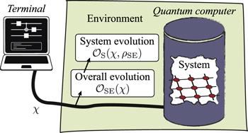
Figure 1. Quantum computer controlled by the state of a terminal. The state of the terminal χ results in the evolution ${{ \mathcal O }}_{\mathrm{SE}}(\chi )$ of the system and environment. The evolution of the system ${{ \mathcal O }}_{{\rm{S}}}(\chi ,{\rho }_{\mathrm{SE}})$ depends on both the terminal state χ and the state of the system and environment at the beginning of the evolution ρSE. |
2.1. State, measurement, operations and Pauli transfer matrix representation
3. Self-consistent tomography without information completeness
3.1. Linear operator tomography
| • | Choose a set of states $\{\left|{\rho }_{i}\right.\unicode{x027EB}={{ \mathcal O }}_{i}\left|{\rho }_{\mathrm{in}}\right.\unicode{x027EB}\}$ and a set of observables $\{\left.\unicode{x027EA}{Q}_{k}\right|=\left.\unicode{x027EA}{Q}_{\mathrm{out}}\right|{{ \mathcal O }}_{k}^{\prime} \}$. Here, ${{ \mathcal O }}_{i},{{ \mathcal O }}_{k}^{\prime} \in O$, i, k = 1, ⋯ ,d and we take d = dV. We always take $\left|{\rho }_{1}\right.\unicode{x027EB}=\left|{\rho }_{\mathrm{in}}\right.\unicode{x027EB}$ and $\left.\unicode{x027EA}{Q}_{1}\right|=\left.\unicode{x027EA}{Q}_{\mathrm{out}}\right|$. |
| • | These states and observables must satisfy the condition that $\{P\left|{\rho }_{i}\right.\unicode{x027EB}\}$ and $\{\left.\unicode{x027EA}{Q}_{k}\right|P\}$ are both linearly independent. According to the definition of the subspace V, states and observables satisfying the condition always exist and can be realised in the quantum computer using the combination of elementary operations. |
| • | Obtain matrices g = MoutMin and $\widetilde{{ \mathcal O }}(\chi )={M}_{\mathrm{out}}{ \mathcal O }(\chi ){M}_{\mathrm{in}}$ for each χ in the experiment. Here, ${M}_{\mathrm{in}}\,=[\ \left|{\rho }_{1}\right.\unicode{x027EB}\ \cdots \ \left|{\rho }_{d}\right.\unicode{x027EB}\ ]$ is the matrix with $\{\left|{\rho }_{i}\right.\unicode{x027EB}\}$ as columns, and ${M}_{\mathrm{out}}={[{\left.\unicode{x027EA}{Q}_{1}\right|}^{{\rm{T}}}\cdots {\left.\unicode{x027EA}{Q}_{d}\right|}^{{\rm{T}}}]}^{{\rm{T}}}$ is the matrix with $\{\left.\unicode{x027EA}{Q}_{k}\right|\}$ as rows. Each matrix element can be measured in the experiment. The element ${g}_{k,i}=\unicode{x027EA}{Q}_{k}| {\rho }_{i}\unicode{x027EB}$ is the mean of Qk in the state ρi. The element ${\widetilde{{ \mathcal O }}}_{k,i}(\chi )\,=\left.\unicode{x027EA}{Q}_{k}\right|{ \mathcal O }(\chi )\left|{\rho }_{i}\right.\unicode{x027EB}$ is the mean ofQk in the state ρi after the operation ${ \mathcal O }(\chi )$. |
| • | When $\{P\left|{\rho }_{i}\right.\unicode{x027EB}\}$ and $\{\left.\unicode{x027EA}{Q}_{k}\right|P\}$ are both linearly independent, g is invertible. We remark that $\{P\left|{\rho }_{i}\right.\unicode{x027EB}\}$ and $\{\left.\unicode{x027EA}{Q}_{k}\right|P\}$ may not be linearly independent when $\{\left|{\rho }_{i}\right.\unicode{x027EB}\}$ and $\{\left.\unicode{x027EA}{Q}_{k}\right|\}$ are linearly independent because of the projection P. |
| • | Choose a d-dimensional invertible real matrix ${\widehat{M}}_{\mathrm{in}}$, and compute ${\widehat{M}}_{\mathrm{out}}=g{\widehat{M}}_{\mathrm{in}}^{-1}$. |
| • | Take $\left|{\widehat{\rho }}_{\mathrm{in}}\right.\unicode{x027EB}={\widehat{M}}_{\mathrm{in};\bullet ,1}$ and $\left.\unicode{x027EA}{\widehat{Q}}_{\mathrm{out}}\right|={\widehat{M}}_{\mathrm{out};1,\bullet }$, and compute $\widehat{{ \mathcal O }}(\chi )={\widehat{M}}_{\mathrm{out}}^{-1}\widetilde{{ \mathcal O }}(\chi ){\widehat{M}}_{\mathrm{in}}^{-1}$ for each χ. |
4. Space dimension truncation
5. Approximate models of temporally correlated errors
5.1. Low-frequency noise and classical random variables
5.1.1. Second-order approximation
5.1.2. High-order approximations and multiple variables
5.2. Classical context-dependent noise
6. Approximate quantum tomography
6.1. Linear inversion method
| • | Choose a set of states $\{\left|{\rho }_{i}^{{\rm{t}}}\right.\unicode{x027EB}={{ \mathcal O }}_{i}\left|{\rho }_{\mathrm{in}}\right.\unicode{x027EB}\,| \,{{ \mathcal O }}_{i}\in O;i\,=1,\cdots ,{d}^{{\rm{t}}}\}$ and a set of observables $\{\left.\unicode{x027EA}{Q}_{k}^{{\rm{t}}}\right|=\left.\unicode{x027EA}{Q}_{\mathrm{out}}\right|{{ \mathcal O }}_{k}^{\prime} \,| \,{{ \mathcal O }}_{k}^{\prime} \,\in O;k=1,\cdots ,{d}^{{\rm{t}}}\}$. We always take $\left|{\rho }_{1}^{{\rm{t}}}\right.\unicode{x027EB}=\left|{\rho }_{\mathrm{in}}\right.\unicode{x027EB}$ and $\left.\unicode{x027EA}{Q}_{1}^{{\rm{t}}}\right|=\left.\unicode{x027EA}{Q}_{\mathrm{out}}\right|$. Here, O is the set of operation sequences. |
| • | Obtain matrices ${g}^{{\rm{t}}}={M}_{\mathrm{out}}^{{\rm{t}}}{M}_{\mathrm{in}}^{{\rm{t}}}$ and ${\widetilde{{ \mathcal O }}}^{{\rm{t}}}(\chi )={M}_{\mathrm{out}}^{{\rm{t}}}{ \mathcal O }(\chi ){M}_{\mathrm{in}}^{{\rm{t}}}$ for each χ in the experiment. Here, ${M}_{\mathrm{in}}^{{\rm{t}}}=[\ \left|{\rho }_{1}^{{\rm{t}}}\right.\unicode{x027EB}\ \cdots \ \left|{\rho }_{{d}^{{\rm{t}}}}^{{\rm{t}}}\right.\unicode{x027EB}\ ]$ and ${M}_{\mathrm{out}}^{{\rm{t}}}={[{\left.\unicode{x027EA}{Q}_{1}^{{\rm{t}}}\right|}^{{\rm{T}}}\cdots {\left.\unicode{x027EA}{Q}_{{d}^{{\rm{t}}}}^{{\rm{t}}}\right|}^{{\rm{T}}}]}^{{\rm{T}}}$. |
| • | Compute the singular value decomposition UgtV = Λ, where ${\rm{\Lambda }}=\mathrm{diag}({s}_{1},{s}_{2},\ldots ,{s}_{{d}^{{\rm{t}}}})$, and singular values are sorted in the descending order ${s}_{1}\geqslant {s}_{2}\geqslant \cdots \geqslant {s}_{{d}^{{\rm{t}}}}$. |
| • | Choose the dimension d. Compute g = diag(s1, s2,…,sd) = DΛD† and $\widetilde{{ \mathcal O }}(\chi )={DU}{\widetilde{{ \mathcal O }}}^{{\rm{t}}}(\chi ){{VD}}^{\dagger }$ for each χ. Here, D is a d × dt matrix, and ${D}_{i,i^{\prime} }={\delta }_{i,i^{\prime} }$. |
| • | Choose a d-dimensional invertible real matrix ${\widehat{M}}_{\mathrm{in}}$, and compute ${\widehat{M}}_{\mathrm{out}}=g{\widehat{M}}_{\mathrm{in}}^{-1}$. |
| • | Compute $\left|{\widehat{\rho }}_{\mathrm{in}}\right.\unicode{x027EB}={\sum }_{i=1}^{d}{\widehat{M}}_{\mathrm{in};\bullet ,{\rm{i}}}{V}_{1,i}^{* }={\widehat{M}}_{\mathrm{out}}^{-1}{{DUg}}_{\bullet ,1}^{{\rm{t}}}$, $\left.\unicode{x027EA}{\widehat{Q}}_{\mathrm{out}}\right|={\sum }_{k=1}^{d}{U}_{k,1}^{* }{\widehat{M}}_{\mathrm{out};{\rm{k}},\bullet }={g}_{1,\bullet }^{{\rm{t}}}{{VD}}^{\dagger }{\widehat{M}}_{\mathrm{in}}^{-1}$, and $\widehat{{ \mathcal O }}(\chi )={\widehat{M}}_{\mathrm{out}}^{-1}\widetilde{{ \mathcal O }}(\chi ){\widehat{M}}_{\mathrm{in}}^{-1}$ for each χ. |
6.2. Maximum likelihood estimation
| • | Parameterize the d-dimensional column vector $\left|{\bar{\rho }}_{\mathrm{in}}({\boldsymbol{x}})\right.\unicode{x027EB}$, row vector $\left.\unicode{x027EA}{\bar{Q}}_{\mathrm{out}}({\boldsymbol{x}})\right|$ and matrix $\bar{{ \mathcal O }}(\chi ,{\boldsymbol{x}})$ for each χ as functions of parameters x = (x1, x2, …). |
| • | Choose M circuits {χ1,…,χM}. For each circuit ${{\boldsymbol{\chi }}}_{m}\,=({\chi }_{m,1},\cdots ,{\chi }_{m,{N}_{m}})$, obtain $\left.\unicode{x027EA}{Q}_{\mathrm{out}}\right|{ \mathcal O }({\chi }_{m,{N}_{m}})\cdots { \mathcal O }({\chi }_{m,1})\left|{\rho }_{\mathrm{in}}\right.\unicode{x027EB}$ in the experiment. The result is Cm. |
| • | Minimize the likelihood function $L({\boldsymbol{x}})={\prod }_{m\,=\,1}^{M}\exp \{-{[{\bar{C}}_{m}({\boldsymbol{x}})-{C}_{m}]}^{2}/{\sigma }_{m}^{2}\}$, where ${\bar{C}}_{m}({\boldsymbol{x}})=\left.\unicode{x027EA}{\bar{Q}}_{\mathrm{out}}({\boldsymbol{x}})\right|\bar{{ \mathcal O }}({\chi }_{m,{N}_{m}},{\boldsymbol{x}})\cdots \bar{{ \mathcal O }}({\chi }_{m,1},{\boldsymbol{x}})\left|{\bar{\rho }}_{\mathrm{in}}({\boldsymbol{x}})\right.\unicode{x027EB}$, and ${\sigma }_{m}^{2}$ is the variance of Cm. The likelihood function is minimized at $\widehat{{\boldsymbol{x}}}=\arg \ {\min }_{{\boldsymbol{x}}}\{L({\boldsymbol{x}})\}$. |
| • | Compute $\left|{\widehat{\rho }}_{\mathrm{in}}\right.\unicode{x027EB}=\left|{\bar{\rho }}_{\mathrm{in}}(\widehat{{\boldsymbol{x}}})\right.\unicode{x027EB}$, $\left.\unicode{x027EA}{\widehat{Q}}_{\mathrm{out}}\right|=\left.\unicode{x027EA}{\bar{Q}}_{\mathrm{out}}(\widehat{{\boldsymbol{x}}})\right|$, and $\widehat{{ \mathcal O }}(\chi )=\bar{{ \mathcal O }}(\chi ,\widehat{{\boldsymbol{x}}})$ for each χ. |
7. Numerical simulation of low-frequency noise
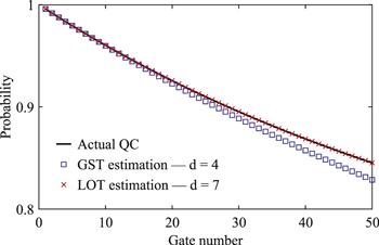
Figure 2. Probabilities in the state $\left|0\right|$ after a sequence of randomly chosen Hadamard and phase gates as functions of the gate number. We initialize the qubit in the state $\left|0\right|$, perform the random gate sequence and measure the probability in the state $\left|0\right|$. We only take into account gate sequences that the final state is $\left|0\right|$ in the case of ideal gates without error. Therefore the probability should be 1 in this case. In our simulation, we take Σ = 1 and η = 0.02. In the presence of errors, the probability in the actual quantum computation (QC) decreases with the gate number (black curve). Based on error models obtained in linear operator tomography (LOT) using MLE, we can estimate the decreasing probability, and the results are plotted. We can find the that the error model with d = 7 (red crosses) fits the actual behavior of the quantum computer much more accurately than the error model with d = 4 (blue squares). When d = 4, LOT is equivalent to conventional GST. Results for the linear inversion method are similar. See appendix |
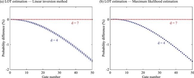
$\sigma ,\ \ \tau ={I}_{{\rm{S}}}\otimes {\rho }_{{\rm{E}}}^{{\rm{a}}}/\sqrt{a},\ {X}_{{\rm{S}}}\otimes \left|1\right\rangle {\left\langle 1\right|}_{{\rm{E}}}^{{\rm{a}}},\ {Y}_{{\rm{S}}}\otimes \left|1\right\rangle {\left\langle 1\right|}_{{\rm{E}}}^{{\rm{a}}},\ {Z}_{{\rm{S}}}\otimes \left|1\right\rangle {\left\langle 1\right|}_{{\rm{E}}}^{{\rm{a}}},\ {X}_{{\rm{S}}}\otimes \left|2\right\rangle {\left\langle 2\right|}_{{\rm{E}}}^{{\rm{a}}},\ {Y}_{{\rm{S}}}\otimes \left|2\right\rangle {\left\langle 2\right|}_{{\rm{E}}}^{{\rm{a}}},\ {Z}_{{\rm{S}}}\otimes \left|2\right\rangle {\left\langle 2\right|}_{{\rm{E}}}^{{\rm{a}}}$ and $a=\mathrm{Tr}({\rho }_{{\rm{E}}}^{{\rm{a}}2})$. Pauli transfer matrices obtained using LIM are show in figure 3. In figure 4, we show the error in probabilities in the ideal state ∣0> estimated using different methods.
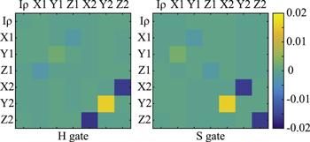
Figure 3. Pauli transfer matrices obtained using the linear inversion method. The difference between the matrix obtained in tomography and the matrix of the ideal gate, i.e. ${M}_{{ \mathcal O }}-{M}_{{ \mathcal O }}^{\mathrm{ideal}}$, is plotted. See appendix |
Figure 4. The difference between probabilities in the ideal state $\left|0\right|$ after a sequence of randomly chosen gates. (a,b) The probability difference Ftom − Fact, where Fact is the probability obtained in the actual quantum computing, and Ftom is the probability estimated using linear operator tomography (LOT). The errorbar denotes one standard deviation. |
8. Conclusions
Appendix A. Exact LOT
Let ${ \mathcal O }\in O$, all the following expressions are valid.
We have
Using ${ \mathcal O }{P}_{\mathrm{in}}={P}_{\mathrm{in}}{ \mathcal O }{P}_{\mathrm{in}}$ and ${P}_{\mathrm{out}}{ \mathcal O }={P}_{\mathrm{out}}{ \mathcal O }{P}_{\mathrm{out}}$, we have
Let $\left|\sigma \right.\unicode{x027EB}\in {V}_{\mathrm{in}}$, $\left.\unicode{x027EA}H\right|\in {V}_{\mathrm{out}}$ and ${{ \mathcal O }}_{i}\in O$, where $i=1,2,\ldots ,N$. Then,
Using lemma
Using $\left|\sigma \right.\unicode{x027EB}={P}_{\mathrm{in}}\left|\sigma \right.\unicode{x027EB}$ and $\left.\unicode{x027EA}H\right|=\left.\unicode{x027EA}H\right|{P}_{\mathrm{out}}$, we have
Let $d=\mathrm{Tr}(P)$, and each of $\{P\left|{\rho }_{i}\right.\unicode{x027EB}\}$ and $\{\left.\unicode{x027EA}{Q}_{k}\right|P\}$ be a set of d linearly-independent vectors. Then, $g={M}_{\mathrm{out}}{M}_{\mathrm{in}}={M}_{\mathrm{out}}{{PM}}_{\mathrm{in}}$ is invertible, $\widetilde{{ \mathcal O }}={M}_{\mathrm{out}}{ \mathcal O }{M}_{\mathrm{in}}\,={M}_{\mathrm{out}}P{ \mathcal O }{{PM}}_{\mathrm{in}}$ and
We remark that $P={\hat{P}}_{\mathrm{out}}$, and the theorem is also valid for ${\hat{P}}_{\mathrm{in}}$.
According to definitions of ${M}_{\mathrm{out}}$ and ${M}_{\mathrm{in}}$, we have ${g}_{k,i}=\unicode{x027EA}{Q}_{k}| {\rho }_{i}\unicode{x027EB}$. Because $\left|{\rho }_{i}\right.\unicode{x027EB}\in {V}_{\mathrm{in}}$ and $\left.\unicode{x027EA}{Q}_{k}\right|\in {V}_{\mathrm{out}}$, we have ${g}_{k,i}=\left.\unicode{x027EA}{Q}_{k}\right|{\hat{P}}_{\mathrm{in}}\left|{\rho }_{i}\right.\unicode{x027EB}=\left.\unicode{x027EA}{Q}_{k}\right|{\hat{P}}_{\mathrm{out}}\left|{\rho }_{i}\right.\unicode{x027EB}$. Here, we have used theorem
Similarly, we have ${\widetilde{{ \mathcal O }}}_{k,i}=\left.\unicode{x027EA}{Q}_{k}\right|{ \mathcal O }\left|{\rho }_{i}\right.\unicode{x027EB}=\left.\unicode{x027EA}{Q}_{k}\right|{\hat{P}}_{\mathrm{in}}{ \mathcal O }{\hat{P}}_{\mathrm{in}}\left|{\rho }_{i}\right.\unicode{x027EB}\,=\left.\unicode{x027EA}{Q}_{k}\right|{\hat{P}}_{\mathrm{out}}{ \mathcal O }{\hat{P}}_{\mathrm{out}}\left|{\rho }_{i}\right.\unicode{x027EB}$. Therefore, ${M}_{\mathrm{out}}{ \mathcal O }{M}_{\mathrm{in}}={M}_{\mathrm{out}}P{ \mathcal O }{{PM}}_{\mathrm{in}}$
We also have
${{PM}}_{\mathrm{in}}$ is a full rank ${d}_{{\rm{H}}}^{2}\times \mathrm{Tr}(P)$ matrix, and ${M}_{\mathrm{out}}P$ is a full rank $\mathrm{Tr}(P)\times {d}_{{\rm{H}}}^{2}$ matrix. Thus, ${\left({{PM}}_{\mathrm{in}}\right)}^{+}{{PM}}_{\mathrm{in}}={\mathbb{1}}$, ${{PM}}_{\mathrm{in}}{\left({{PM}}_{\mathrm{in}}\right)}^{+}=P$, ${M}_{\mathrm{out}}P{\left({M}_{\mathrm{out}}P\right)}^{+}={\mathbb{1}}$ and ${\left({M}_{\mathrm{out}}P\right)}^{+}{M}_{\mathrm{out}}P\,=P$. Here, ${A}^{+}$ denotes the pseudo inverse of matrix A.
Using pseudo inverses, we have ${g}^{-1}={\left({{PM}}_{\mathrm{in}}\right)}^{+}{\left({M}_{\mathrm{out}}P\right)}^{+}$, i.e. $g={M}_{\mathrm{out}}{{PPM}}_{\mathrm{in}}$ is invertible. Thus,
Appendix B. Space dimension truncation
Let ${N}_{Q}\geqslant \parallel \left.\unicode{x027EA}{Q}_{k}\right|\parallel $ for all k, and ${N}_{\rho }\geqslant \parallel \left|{\rho }_{i}\right.\unicode{x027EB}\parallel $ for all i. Then
Let ${N}_{Q}\geqslant \parallel \left.\unicode{x027EA}{Q}_{k}\right|\parallel $ for all k, and ${N}_{\rho }\geqslant \parallel \left|{\rho }_{i}\right.\unicode{x027EB}\parallel $ for all i. Then, for any sequence of operations,
Inequality (
If inequality (
Appendix C. Linear inversion method
$\{\left|{\rho }_{i}^{{\rm{a}}}\right.\unicode{x027EB}\}$ are columns of ${M}_{\mathrm{in}}^{{\rm{a}}}$, and $\{\left.\unicode{x027EA}{Q}_{k}^{{\rm{a}}}\right|\}$ are rows of ${M}_{\mathrm{out}}^{{\rm{a}}}$. Let ${N}_{Q}^{{\rm{a}}}\geqslant \parallel \left.\unicode{x027EA}{Q}_{k}^{{\rm{a}}}\right|\parallel $ for all k, and ${N}_{\rho }^{{\rm{a}}}\geqslant \parallel \left|{\rho }_{i}^{{\rm{a}}}\right.\unicode{x027EB}\parallel $ for all i. If g, ${M}_{\mathrm{in}}^{{\rm{a}}}$ and ${M}_{\mathrm{out}}^{{\rm{a}}}$ are inevitable, for any sequence of operations in $\{{ \mathcal O }(\chi )\}$,
We have