


1. Introduction
The soliton is one of the most notable characteristics that characterize the integrability of the nonlinear evolution equation [1, 2]. Recently, stray or monster waves, weird waves, and abnormal waves have been regarded as solitary waves. Solitary waves are an uncommon type of nonlinear wave that is restricted in only one direction and has important significance in various branches of physics [3, 4]. These waves were first found in the deep sea [5]. The applications of this wave appear in oceanography and optical fibers [6, 7]. Nowadays, a new type of wandering wave is known as the lumped wave, which is defined as a wave whose wandering is restricted in each direction in space [8].
Nowadays, based on the computer revolution, which has a great effect on the derivation of computational, semi-analytical, and numerical schemes, many schemes have derived, such as the sech-tanh expansion method, the auxiliary equation method, the direct algebraic equation method, the iteration method, the exponential expansion method, B-spline schemes, Kudryashov methods, the Adomian decomposition method, Khater methods, $\left(\tfrac{\varphi ^{\prime} (\zeta )}{\varphi (\zeta )}\right)$- expansion methods, and so on [9–15]; in addition, the lump solutions of many nonlinear phenomena have been investigated [16–20].
In this context, our paper aims to study the new soliton-wave solutions of the generalized CBS equation through the perspective of ESE, and MKud analysis technology [21, 22]. Another goal of the manuscript is to limit the examination of the semi-analytical and numerical solutions of the considered model to an explanation of the accuracy of the analytical solutions obtained and the analytical schemes used [23, 24]. The generalized CBS equation is given by [25–30]:2 ) is given in (2+1) dimensions, and has the following formula2 ) was derived by Bogoyavlenskii and Schiff in different ways, such as the modified Lax formalism and a reduction of the self-dual Yang–Mills equation. Additionally, the nonlocal form of the (2+1)-dimensional model is given by2 ), (4 ), and (5 ) describe many nonlinear phenomena in plasma physics. Employing the next wave transformation ${ \mathcal C }={ \mathcal C }(x,y,t)={ \mathcal S }({\mathfrak{P}})$, where ${\mathfrak{P}}={r}_{1}x+{r}_{2}y\,+{r}_{3}t$ and ri, i = 1, 2, 3 are arbitrary constants, converts equation (2 ) into the following ordinary differential equation. Integrating the obtained equation once with the zero constant of integration, we get:6 ) through the perspective of the abovementioned analytical schemes and the homogeneous balance principle gives n = 1. Thus, the general solutions of equation (6 ) are evaluated by
$\begin{eqnarray}{{ \mathcal B }}_{t}+{{ \mathcal B }}_{{xxy}}+3{ \mathcal B }{{ \mathcal B }}_{y}+3{{ \mathcal B }}_{x}{{ \mathcal C }}_{y}+{r}_{1}{{ \mathcal B }}_{y}+{r}_{2}{{ \mathcal C }}_{{yy}}=0,\end{eqnarray}$
where ${ \mathcal B }={ \mathcal B }(x,t,t),{ \mathcal C }={ \mathcal C }(x,y,t)$ describe the dynamics of solitons and nonlinear waves, while ri, i = 1, 2 are arbitrary constants to be determined later. Using the next relation between ${ \mathcal C }\ \& \ { \mathcal B }$ in the following formula, ${ \mathcal B }={{ \mathcal C }}_{x}$, yields $\begin{eqnarray}{{ \mathcal C }}_{{tx}}+{{ \mathcal C }}_{{xxxy}}+3{{ \mathcal C }}_{x}{{ \mathcal C }}_{{xy}}+3{{ \mathcal C }}_{{xx}}{{ \mathcal C }}_{y}=0.\end{eqnarray}$
Eq. ( $\begin{eqnarray}{{ \mathcal B }}_{t}+{ \mathcal B }{{ \mathcal B }}_{z}+\displaystyle \frac{1}{2}{{ \mathcal B }}_{x}{\partial }_{x}^{-1}{{ \mathcal B }}_{z}+\displaystyle \frac{1}{4}{{ \mathcal B }}_{{xxz}}=0,\end{eqnarray}$
where ${\partial }_{x}^{-1}{{ \mathcal B }}_{z}=\in {{ \mathcal B }}_{z}{dx}$. Equation ( $\begin{eqnarray}\left\{\begin{array}{c}{{ \mathcal C }}_{x}-{{ \mathcal B }}_{z}=0,\\ 2{{ \mathcal B }}_{x}{ \mathcal C }+{{ \mathcal B }}_{{xxz}}+4{{ \mathcal B }}_{t}+4{ \mathcal B }{{ \mathcal B }}_{z}=0,\end{array}\right.\end{eqnarray}$
while the potential form is given by $\begin{eqnarray}4{{ \mathcal E }}_{{tx}}+4{{ \mathcal E }}_{x}{{ \mathcal E }}_{{xz}}+2{{ \mathcal E }}_{{xx}}{{ \mathcal E }}_{z}+{{ \mathcal E }}_{{xxxz}}=0.\end{eqnarray}$
Equations ( $\begin{eqnarray}{r}_{3}{{ \mathcal S }}^{{\prime} }+{r}_{2}{r}_{1}^{2}{{ \mathcal S }}^{(3)}+3{r}_{2}{r}_{1}{\left({{ \mathcal S }}^{{\prime} }\right)}^{2}=0.\end{eqnarray}$
Handling equation ( $\begin{eqnarray}{ \mathcal S }({\mathfrak{P}})=\left\{\begin{array}{c}{\sum }_{i=-n}^{n}{a}_{i}{\mathfrak{C}}{\left({\mathfrak{P}}\right)}^{i}={a}_{1}{\mathfrak{C}}({\mathfrak{P}})+\displaystyle \frac{{a}_{-1}}{{\mathfrak{C}}({\mathfrak{P}})}+{a}_{0},\\ {\sum }_{i=0}^{n}{a}_{i}{\mathfrak{L}}{\left({\mathfrak{P}}\right)}^{i}={a}_{1}{\mathfrak{L}}({\mathfrak{P}})+{a}_{0},\end{array}\right.\end{eqnarray}$
where a0, a1, and a−1 are arbitrary constants.The other sections of this manuscript are as follows: section 2 studies the general solution of the generalized CBS model. In addition, the accuracy of the obtained solution is checked using the abovementioned semi-analytical scheme. Section 3 introduces the solutions and achieves the goals of our research paper. Section 4 provides a summary of the manuscript.
2. Comparison of analytical and semi-analytical approaches to the generalized CBS equation
This section studies the analytical, semi-analytical, and numerical simulation of the generalized CBS equation. The headings of this section can be summarized in the following order:
| • | We apply the ESE and MKud schemes to equation ( |
| • | We check the accuracy of the obtained solution and calculate the absolute error value between the exact and semi-analytical solutions. |
2.1. ESE analytical vs. VI numerical techniques, along with the generalized CBS equation
Applying the ESE scheme’s framework and its auxiliary, $\left({{\mathfrak{C}}}^{{\prime} }({\mathfrak{P}})={h}_{3}{\mathfrak{C}}{\left({\mathfrak{P}}\right)}^{2}+{h}_{2}{\mathfrak{C}}({\mathfrak{P}})+{h}_{1}\right)$ (where hi, i = 1, 2, 3 are arbitrary constants to be determined later), to equation (6 ) obtains the following sets of abovementioned parameters:
Set I
$\begin{eqnarray*}{a}_{-1}\to \displaystyle \frac{2{h}_{1}}{{r}_{1}},{a}_{1}\to 0,{r}_{3}\to -\left({h}_{2}^{2}-4{h}_{1}{h}_{3}\right){r}_{2}.\end{eqnarray*}$
Set II
$\begin{eqnarray*}{a}_{-1}\to 0,{a}_{1}\to -\displaystyle \frac{2{h}_{3}}{{r}_{1}},{r}_{3}\to -\left({h}_{2}^{2}-4{h}_{1}{h}_{3}\right){r}_{2}.\end{eqnarray*}$
Therefore, the solitary solutions of the considered model are constructed in the following formulas:For h2 = 0, h1h3 > 0, we get
$\begin{eqnarray}{{ \mathcal C }}_{{\rm{I}},1}={a}_{0}+\displaystyle \frac{2\sqrt{{h}_{1}{h}_{3}}\cot \left(\sqrt{{h}_{1}{h}_{3}}\left(\eta +{r}_{2}\left(4{h}_{1}{h}_{3}t+y\right)+{r}_{1}x\right)\right)}{{r}_{1}},\end{eqnarray}$
$\begin{eqnarray}{{ \mathcal C }}_{{\rm{I}},2}={a}_{0}+\displaystyle \frac{2\sqrt{{h}_{1}{h}_{3}}\tan \left(\sqrt{{h}_{1}{h}_{3}}\left(\eta +{r}_{2}\left(4{h}_{1}{h}_{3}t+y\right)+{r}_{1}x\right)\right)}{{r}_{1}},\end{eqnarray}$
$\begin{eqnarray}{{ \mathcal C }}_{\mathrm{II},1}={a}_{0}-\displaystyle \frac{2\sqrt{{h}_{1}{h}_{3}}\tan \left(\sqrt{{h}_{1}{h}_{3}}\left(\eta +{r}_{2}\left(4{h}_{1}{h}_{3}t+y\right)+{r}_{1}x\right)\right)}{{r}_{1}},\end{eqnarray}$
$\begin{eqnarray}{{ \mathcal C }}_{\mathrm{II},2}={a}_{0}-\displaystyle \frac{2\sqrt{{h}_{1}{h}_{3}}\cot \left(\sqrt{{h}_{1}{h}_{3}}\left(\eta +{r}_{2}\left(4{h}_{1}{h}_{3}t+y\right)+{r}_{1}x\right)\right)}{{r}_{1}}.\end{eqnarray}$
For h2 = 0, h1h3 < 0, we get
$\begin{eqnarray}{{ \mathcal C }}_{{\rm{I}},3}={a}_{0}-\displaystyle \frac{2\sqrt{-{h}_{1}{h}_{3}}\coth \left(\sqrt{-{h}_{1}{h}_{3}}\left({r}_{2}\left(4{h}_{1}{h}_{3}t+y\right)+{r}_{1}x\right)\mp \tfrac{\mathrm{log}(\eta )}{2}\right)}{{r}_{1}},\end{eqnarray}$
$\begin{eqnarray}{{ \mathcal C }}_{{\rm{I}},4}={a}_{0}-\displaystyle \frac{2\sqrt{-{h}_{1}{h}_{3}}\tanh \left(\sqrt{-{h}_{1}{h}_{3}}\left({r}_{2}\left(4{h}_{1}{h}_{3}t+y\right)+{r}_{1}x\right)\mp \tfrac{\mathrm{log}(\eta )}{2}\right)}{{r}_{1}},\end{eqnarray}$
$\begin{eqnarray}{{ \mathcal C }}_{\mathrm{II},3}={a}_{0}-\displaystyle \frac{2\sqrt{-{h}_{1}{h}_{3}}\tanh \left(\sqrt{-{h}_{1}{h}_{3}}\left({r}_{2}\left(4{h}_{1}{h}_{3}t+y\right)+{r}_{1}x\right)\mp \tfrac{\mathrm{log}(\eta )}{2}\right)}{{r}_{1}},\end{eqnarray}$
$\begin{eqnarray}{{ \mathcal C }}_{\mathrm{II},4}={a}_{0}-\displaystyle \frac{2\sqrt{-{h}_{1}{h}_{3}}\coth \left(\sqrt{-{h}_{1}{h}_{3}}\left({r}_{2}\left(4{h}_{1}{h}_{3}t+y\right)+{r}_{1}x\right)\mp \tfrac{\mathrm{log}(\eta )}{2}\right)}{{r}_{1}}.\end{eqnarray}$
For h1 = 0, h2 > 0, we get
$\begin{eqnarray}{{ \mathcal C }}_{\mathrm{II},5}={a}_{0}+\displaystyle \frac{2{h}_{2}}{{r}_{1}\left({h}_{3}{e}^{{h}_{2}\left(\eta +{r}_{2}\left(y-{h}_{2}^{2}t\right)+{r}_{1}x\right)}-1\right)}+\displaystyle \frac{2{h}_{2}}{{r}_{1}}.\end{eqnarray}$
For h1 = 0, h2 < 0, we get
$\begin{eqnarray}{{ \mathcal C }}_{\mathrm{II},6}={a}_{0}-\displaystyle \frac{2{h}_{3}}{{r}_{1}\left({h}_{3}{e}^{{h}_{2}\left(\eta +{r}_{2}\left(y-{h}_{2}^{2}t\right)+{r}_{1}x\right)}+1\right)}+\displaystyle \frac{2{h}_{3}}{{r}_{1}}.\end{eqnarray}$
For $4{h}_{1}{h}_{3}\gt {h}_{2}^{2}$, we get
$\begin{eqnarray}{{ \mathcal C }}_{{\rm{I}},5}={a}_{0}-\displaystyle \frac{4{h}_{1}{h}_{3}}{{r}_{1}\left({h}_{2}-\sqrt{4{h}_{1}{h}_{3}-{h}_{2}^{2}}\tan \left(\tfrac{1}{2}\sqrt{4{h}_{1}{h}_{3}-{h}_{2}^{2}}\left(\eta +{r}_{2}\left({h}_{2}^{2}(-t)+4{h}_{1}{h}_{3}t+y\right)+{r}_{1}x\right)\right)\right)},\end{eqnarray}$
$\begin{eqnarray}{{ \mathcal C }}_{{\rm{I}},6}={a}_{0}-\displaystyle \frac{4{h}_{1}{h}_{3}}{{r}_{1}\left({h}_{2}-\sqrt{4{h}_{1}{h}_{3}-{h}_{2}^{2}}\cot \left(\tfrac{1}{2}\sqrt{4{h}_{1}{h}_{3}-{h}_{2}^{2}}\left(\eta +{r}_{2}\left({h}_{2}^{2}(-t)+4{h}_{1}{h}_{3}t+y\right)+{r}_{1}x\right)\right)\right)},\end{eqnarray}$
$\begin{eqnarray}{{ \mathcal C }}_{\mathrm{II},7}={a}_{0}-\displaystyle \frac{\sqrt{4{h}_{1}{h}_{3}-{h}_{2}^{2}}\tan \left(\tfrac{1}{2}\sqrt{4{h}_{1}{h}_{3}-{h}_{2}^{2}}\left(\eta +{r}_{2}\left({h}_{2}^{2}(-t)+4{h}_{1}{h}_{3}t+y\right)+{r}_{1}x\right)\right)}{{r}_{1}}+\displaystyle \frac{{h}_{2}}{{r}_{1}},\end{eqnarray}$
$\begin{eqnarray}{{ \mathcal C }}_{\mathrm{II},8}={a}_{0}-\displaystyle \frac{\sqrt{4{h}_{1}{h}_{3}-{h}_{2}^{2}}\cot \left(\tfrac{1}{2}\sqrt{4{h}_{1}{h}_{3}-{h}_{2}^{2}}\left(\eta +{r}_{2}\left({h}_{2}^{2}(-t)+4{h}_{1}{h}_{3}t+y\right)+{r}_{1}x\right)\right)}{{r}_{1}}+\displaystyle \frac{{h}_{2}}{{r}_{1}}.\end{eqnarray}$
2.1.1. Comparison of the analytical and numerical solutions
Applying the VI method to equation (2 ), we get the following semi-analytical solutions:22 ),
$\begin{eqnarray}\begin{array}{rcl}{{ \mathcal C }}_{n+1} & = & {{ \mathcal C }}_{n}-{\displaystyle \int }_{0}^{t}\left(-{\left({{ \mathcal C }}_{n}\right)}_{{xs}}+{\left({{ \mathcal C }}_{n}\right)}_{{xxxz}}\right.\\ & & \left.+4{\left({{ \mathcal C }}_{n}\right)}_{x}{\left({{ \mathcal C }}_{n}\right)}_{{xz}}+2{\left({{ \mathcal C }}_{n}\right)}_{{xx}}{\left({{ \mathcal C }}_{n}\right)}_{z}+3{\left({{ \mathcal C }}_{n}\right)}_{{yy}}\right){ds}.\end{array}\end{eqnarray}$
Using equation ( $\begin{eqnarray}{{ \mathcal C }}_{0}=1-2\tanh (x+2y),\end{eqnarray}$
$\begin{eqnarray}\begin{array}{l}{{ \mathcal C }}_{1}(\zeta ,t)=1-2\tanh (x+2y)\\ \quad \times \left(8t\left(\cosh (2(x+2y))-11\right){{\rm{sech}} }^{4}(x+2y)+1\right),\end{array}\end{eqnarray}$
$\begin{eqnarray}\begin{array}{l}{{ \mathcal C }}_{2}(\zeta ,t)=2{\rm{sech}} (x)\sinh (2y){\rm{sech}} (x+2y)\\ \quad \times \left(32t{{\rm{sech}} }^{2}(x+2y)\left(2{{\rm{sech}} }^{2}(x+2y)\left(12t{{\rm{sech}} }^{2}(x+2y)\right.\right.\right.\\ \quad \times \left(9056t-270){{\rm{sech}} }^{2}(x+2y)-3600t\left(3\cosh (2(x+2y))-1\right)\right.\\ \quad \left.\left.\left.\left.\times {{\rm{sech}} }^{6}(x+2y)-864t+243\right)+4t(64t-117)+3\right)+8t-1\right)-1\right)\\ \quad +2\tanh (x)\left(32t{{\rm{sech}} }^{2}(x+2y)\left(2{{\rm{sech}} }^{2}(x+2y)\right.\right.\\ \quad \times \left(12t{{\rm{sech}} }^{2}(x+2y)\left(9056t-270){{\rm{sech}} }^{2}(x+2y)\right.\right.\\ \quad \left.-3600t\left(3\cosh (2(x+2y))-1\right){{\rm{sech}} }^{6}(x+2y)-864t+243\right)\\ \quad \left.\left.\left.+4t(64t-117)+3\right)+8t-1\right)-1\right)+1.\end{array}\end{eqnarray}$
Using same steps, we can get ${{ \mathcal C }}_{i}$, i = 3, 4, 5, ⋯.2.2. MKud analytical vs. VI numerical techniques, along with the generalized CBS equation
Applying the MKud scheme’s framework and its auxiliary, $\left({{\mathfrak{L}}}^{{\prime} }({\mathfrak{P}})=\mathrm{ln}(k)\left({\mathfrak{L}}{\left({\mathfrak{P}}\right)}^{2}-{\mathfrak{L}}({\mathfrak{P}})\right)\right)$ (where k is an arbitrary constant to be evaluated later), to equation (6 ) obtains the following sets of abovementioned parameters:
Set I
$\begin{eqnarray*}{a}_{1}\to -\displaystyle \frac{2\mathrm{log}(k)}{{r}_{1}},{r}_{3}\to {r}_{2}\left(-{\mathrm{log}}^{2}(k)\right).\end{eqnarray*}$
Therefore, the solitary solutions of the considered model are constructed in the following formula: $\begin{eqnarray}{ \mathcal C }={a}_{0}-\displaystyle \frac{2\mathrm{log}(k)}{{r}_{1}\left(1\pm {k}^{{r}_{2}\left(y-t{\mathrm{log}}^{2}(k)\right)+{r}_{1}x}\right)}.\end{eqnarray}$
2.2.1. Comparison of the analytical and semi-analytical solutions
Applying the VI method along with equation (22 ) to equation (2 ), one obtains
$\begin{eqnarray}{{ \mathcal C }}_{0}=3-\displaystyle \frac{2}{{e}^{x+2y}+1},\end{eqnarray}$
$\begin{eqnarray}\begin{array}{rcl}{{ \mathcal C }}_{1} & = & \displaystyle \frac{1}{{\left({{\rm{e}}}^{x+2y}+1\right)}^{3}}\\ & & \times \left({{\rm{e}}}^{x+2y}\left({{\rm{e}}}^{x+2y}\left(4t+3{{\rm{e}}}^{x+2y}+7\right)-4t+5\right)+1\right),\end{array}\end{eqnarray}$
$\begin{eqnarray}\begin{array}{rcl}{{ \mathcal C }}_{2} & = & \frac{1}{{\left({{\rm{e}}}^{x+2y}+1\right)}^{9}}\left({{\rm{e}}}^{x+2y}\left(\left(4t\left(896{t}^{2}-77t+10\right)+266\right)\right.\right.\\ & & \times {{\rm{e}}}^{4x+8y}+\left(238-4t\left(896{t}^{2}-77t+10\right)\right)\\ & & \times {{\rm{e}}}^{3x+6y}+(25-4(t-2)t){{\rm{e}}}^{7(x+2y)}\\ & & -4\left(3t(5t(16t+3)-6)-49\right){{\rm{e}}}^{5(x+2y)}\\ & & +4\left(3t(5t(16t+3)-6)+35\right){{\rm{e}}}^{2x+4y}\\ & & -4\left(t(t(16t+31)+10)-13\right){{\rm{e}}}^{x+2y}\\ & & +4\left(t(t(16t+31)+10)+23\right){{\rm{e}}}^{6(x+2y)}\\ & & \left.\left.+4(t-2)t+3{{\rm{e}}}^{8(x+2y)}+11\right)+1\right).\end{array}\end{eqnarray}$
Using same steps, we can get ${{ \mathcal C }}_{i}$, i = 3, 4, 5, ⋯.3. Interpretation of the results
This section highlights the novelty of our research papers. It also shows the accuracy of the analytical solution obtained. The ESE and MKud calculation schemes have been applied to the generalized CBS equation for the constructed solitary-wave solution. Many different wave solutions have been obtained, some of which are demonstrated in 2D, 3D, and some sketches in profile drawings to explain solitary waves’ dynamic behavior in nonlinear phenomena in plasma physics. Figures 1 and 3 show the periodic-kink solitary-wave solution. While figure 2 show the semi-analytical solution in three different forms (2D, 3D, and contour plots). Comparing our solution with the solutions obtained in previously published papers, it can be seen that our solution is completely different from the solution evaluated in [25–29].

Figure 1. Solitary-wave-solution equation ( |

Figure 2. Semi-analytical solutions of equation ( |
The VI scheme was applied to the considered model based on the computational solution obtained. The absolute error between the analytical and semi-analytic solutions was calculated, to show the accuracy of the solution and the method used (tables 1 and 2 and figures 3 and 4). This calculation shows that the MKud method is superior to the ESE method, and its absolute error value is much smaller than the absolute value obtained by the ESE method (figure 5).
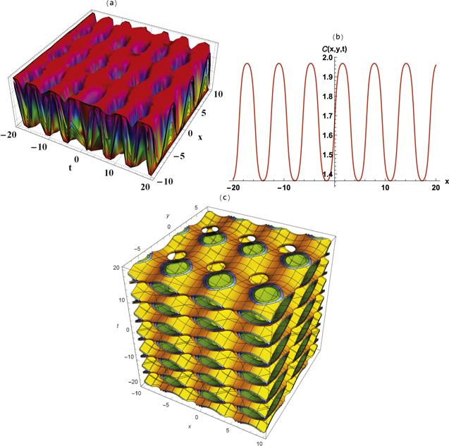
Figure 3. Solitary-wave solutions of equation ( |

Figure 4. Semi-analytical solutions of equation ( |

Figure 5. Absolute errors between the ESE and MKud analytical schemes and the TQBS numerical scheme. |
Table 1. Absolute errors between the analysis obtained using the ESE method and the constructed semi-analytical solution using the VI scheme for different values of x and the following values of the abovementioned parameters: a0 = 1, h2 = 0, h1 = −1, h3 = 1, r1 = −1, and r2 = −2. |
| Value of x | t = 1 | t = 2 | t = 3 | t = 4 | t = 5 | t = 6 | t = 7 | t = 8 | t = 9 | t = 10 |
|---|---|---|---|---|---|---|---|---|---|---|
| 0 | 0.071 941 14 | 3.999 959 59 | 3.999 963 58 | 3.999 934 56 | 3.999 897 1 | 3.999 851 19 | 3.999 796 84 | 3.999 734 05 | 3.999 662 819 | 3.999 583 142 |
| 1 | 0.009 889 99 | 3.999 816 27 | 3.999 995 07 | 3.999 991 14 | 3.999 986 07 | 3.999 979 86 | 3.999 972 51 | 3.999 964 01 | 3.999 954 368 | 3.999 943 585 |
| 2 | 0.001 341 33 | 3.998 658 31 | 3.999 999 33 | 3.999 998 8 | 3.999 998 12 | 3.999 997 27 | 3.999 996 28 | 3.999 995 13 | 3.999 993 824 | 3.999 992 365 |
| 3 | 0.000 181 58 | 3.990 109 47 | 3.999 999 91 | 3.999 999 84 | 3.999 999 74 | 3.999 999 63 | 3.999 999 5 | 3.999 999 34 | 3.999 999 164 | 3.999 998 967 |
| 4 | 2.4575E-05 | 3.928 055 15 | 3.999 999 98 | 3.999 999 98 | 3.999 999 97 | 3.999 999 95 | 3.999 999 93 | 3.999 999 91 | 3.999 999 887 | 3.999 999 86 |
| 5 | 3.3259E-06 | 3.523 188 31 | 3.999 999 94 | 4 | 4 | 3.999 999 99 | 3.999 999 99 | 3.999 999 99 | 3.999 999 985 | 3.999 999 981 |
| 6 | 4.5012E-07 | 2 | 3.999 999 55 | 4 | 4 | 4 | 4 | 4 | 3.999 999 998 | 3.999 999 997 |
| 7 | 6.0917E-08 | 0.476 811 69 | 3.999 996 67 | 4 | 4 | 4 | 4 | 4 | 4 | 4 |
| 8 | 8.2442E-09 | 0.071 944 84 | 3.999 975 42 | 4 | 4 | 4 | 4 | 4 | 4 | 4 |
| 9 | 1.1157E-09 | 0.009 890 49 | 3.999 818 41 | 4 | 4 | 4 | 4 | 4 | 4 | 4 |
| 10 | 1.51E-10 | 0.001 341 4 | 3.998 658 6 | 4 | 4 | 4 | 4 | 4 | 4 | 4 |
| 11 | 2.0435E-11 | 0.000 181 59 | 3.990 109 51 | 4 | 4 | 4 | 4 | 4 | 4 | 4 |
| 12 | 2.7656E-12 | 2.4577E-05 | 3.928 055 16 | 3.999 999 99 | 4 | 4 | 4 | 4 | 4 | 4 |
| 13 | 3.7437E-13 | 3.3261E-06 | 3.523 188 31 | 3.999 999 94 | 4 | 4 | 4 | 4 | 4 | 4 |
| 14 | 5.0626E-14 | 4.5014E-07 | 2 | 3.999 999 55 | 4 | 4 | 4 | 4 | 4 | 4 |
| 15 | 6.8834E-15 | 6.092E-08 | 0.476 811 69 | 3.999 996 67 | 4 | 4 | 4 | 4 | 4 | 4 |
| 16 | 8.8818E-16 | 8.2446E-09 | 0.071 944 84 | 3.999 975 42 | 4 | 4 | 4 | 4 | 4 | 4 |
| 17 | 2.2204E-16 | 1.1158E-09 | 0.009 890 49 | 3.999 818 41 | 4 | 4 | 4 | 4 | 4 | 4 |
| 18 | 0 | 1.5101E-10 | 0.001 341 4 | 3.998 658 6 | 4 | 4 | 4 | 4 | 4 | 4 |
| 19 | 0 | 2.0436E-11 | 0.000 181 59 | 3.990 109 51 | 4 | 4 | 4 | 4 | 4 | 4 |
| 20 | 0 | 2.7658E-12 | 2.4577E-05 | 3.928 055 16 | 3.999 999 99 | 4 | 4 | 4 | 4 | 4 |
| 21 | 0 | 3.7437E-13 | 3.3261E-06 | 3.523 188 31 | 3.999 999 94 | 4 | 4 | 4 | 4 | 4 |
| 22 | 0 | 5.0626E-14 | 4.5014E-07 | 2 | 3.999 999 55 | 4 | 4 | 4 | 4 | 4 |
| 23 | 0 | 6.8834E-15 | 6.092E-08 | 0.476 811 69 | 3.999 996 67 | 4 | 4 | 4 | 4 | 4 |
| 24 | 0 | 8.8818E-16 | 8.2446E-09 | 0.071 944 84 | 3.999 975 42 | 4 | 4 | 4 | 4 | 4 |
| 25 | 0 | 2.2204E-16 | 1.1158E-09 | 0.009 890 49 | 3.999 818 41 | 4 | 4 | 4 | 4 | 4 |
| 26 | 0 | 0 | 1.5101E-10 | 0.001 341 4 | 3.998 658 6 | 4 | 4 | 4 | 4 | 4 |
| 27 | 0 | 0 | 2.0436E-11 | 0.000 181 59 | 3.990 109 51 | 4 | 4 | 4 | 4 | 4 |
| 28 | 0 | 0 | 2.7658E-12 | 2.4577E-05 | 3.928 055 16 | 3.999 999 99 | 4 | 4 | 4 | 4 |
| 29 | 0 | 0 | 3.7437E-13 | 3.3261E-06 | 3.523 188 31 | 3.999 999 94 | 4 | 4 | 4 | 4 |
| 30 | 0 | 0 | 5.0626E-14 | 4.5014E-07 | 2 | 3.999 999 55 | 4 | 4 | 4 | 4 |
Table 2. Absolute errors between the analysis obtained using the MKud method and the constructed semi-analytical solution using the VI scheme for different values of x and the following values of the abovementioned parameters a0 = 1, k = e, r1 = −1, and r2 = −2. |
| Value of x | t = 1 | t = 2 | t = 3 | t = 4 | t = 5 | t = 6 | t = 7 | t = 8 | t = 9 | t = 10 |
|---|---|---|---|---|---|---|---|---|---|---|
| 0 | 0.000 761 9 | 0.004 856 691 | 0.035 343 152 | 0.236 875 694 | 0.997 209 591 | 1.757 184 901 | 1.957 641 682 | 1.986 335 208 | 1.987 919 89 | 1.985 454 506 |
| 1 | 0.000 280 247 | 0.001 789 003 | 0.013 152 735 | 0.094 285 709 | 0.536 850 64 | 1.460 485 799 | 1.902 784 858 | 1.983 386 09 | 1.993 952 21 | 1.994 397 482 |
| 2 | 0.000 103 091 | 0.000 658 453 | 0.004 859 343 | 0.035 763 763 | 0.238 025 35 | 0.999 398 599 | 1.760 722 794 | 1.962 837 217 | 1.993 496 363 | 1.997 353 871 |
| 3 | 3.792 45E-05 | 0.000 242 274 | 0.001 790 473 | 0.013 308 884 | 0.094 711 666 | 0.537 661 43 | 1.461 796 342 | 1.904 709 968 | 1.986 040 478 | 1.997 450 479 |
| 4 | 1.395 15E-05 | 8.913 34E-05 | 0.000 659 061 | 0.004 916 979 | 0.035 920 873 | 0.238 324 368 | 0.999 881 943 | 1.761 432 869 | 1.963 816 413 | 1.994 787 057 |
| 5 | 5.132 47E-06 | 3.279 11E-05 | 0.000 242 507 | 0.001 811 702 | 0.013 366 737 | 0.094 821 77 | 0.537 839 407 | 1.462 057 816 | 1.905 070 56 | 1.986 515 805 |
| 6 | 1.888 13E-06 | 1.206 33E-05 | 8.922 03E-05 | 0.000 666 874 | 0.004 938 269 | 0.035 961 392 | 0.238 389 864 | 0.999 978 169 | 1.761 565 573 | 1.963 991 345 |
| 7 | 6.946 04E-07 | 4.437 85E-06 | 3.282 33E-05 | 0.000 245 382 | 0.001 819 536 | 0.013 381 645 | 0.094 845 868 | 0.537 874 811 | 1.462 106 642 | 1.905 134 923 |
| 8 | 2.5553E-07 | 1.6326E-06 | 1.207 51E-05 | 9.027 79E-05 | 0.000 669 756 | 0.004 943 754 | 0.035 970 257 | 0.238 402 889 | 0.999 996 132 | 1.761 589 252 |
| 9 | 9.400 44E-08 | 6.005 99E-07 | 4.442 21E-06 | 3.321 23E-05 | 0.000 246 442 | 0.001 821 553 | 0.013 384 906 | 0.094 850 659 | 0.537 881 42 | 1.462 115 353 |
| 10 | 3.458 23E-08 | 2.209 48E-07 | 1.6342E-06 | 1.221 83E-05 | 9.066 79E-05 | 0.000 670 498 | 0.004 944 954 | 0.035 972 02 | 0.238 405 321 | 0.999 999 336 |
| 11 | 1.272 21E-08 | 8.128 22E-08 | 6.011 89E-07 | 4.494 87E-06 | 3.335 58E-05 | 0.000 246 715 | 0.001 821 995 | 0.013 385 555 | 0.094 851 554 | 0.537 882 599 |
| 12 | 4.6802E-09 | 2.990 21E-08 | 2.211 65E-07 | 1.653 57E-06 | 1.227 11E-05 | 9.076 84E-05 | 0.000 670 661 | 0.004 945 192 | 0.035 972 349 | 0.238 405 754 |
| 13 | 1.721 75E-09 | 1.100 04E-08 | 8.136 21E-08 | 6.083 15E-07 | 4.514 29E-06 | 3.339 28E-05 | 0.000 246 775 | 0.001 822 082 | 0.013 385 676 | 0.094 851 713 |
| 14 | 6.333 96E-10 | 4.0468E-09 | 2.993 14E-08 | 2.237 87E-07 | 1.660 72E-06 | 1.228 46E-05 | 9.079 04E-05 | 0.000 670 693 | 0.004 945 237 | 0.035 972 408 |
| 15 | 2.330 11E-10 | 1.488 73E-09 | 1.101 12E-08 | 8.232 66E-08 | 6.109 43E-07 | 4.519 29E-06 | 3.340 09E-05 | 0.000 246 786 | 0.001 822 099 | 0.013 385 697 |
| 16 | 8.572 03E-11 | 5.476 75E-10 | 4.050 78E-09 | 3.028 62E-08 | 2.247 54E-07 | 1.662 56E-06 | 1.228 76E-05 | 9.079 47E-05 | 0.000 670 699 | 0.004 945 245 |
| 17 | 3.1537E-11 | 2.0148E-10 | 1.4902E-09 | 1.114 17E-08 | 8.268 22E-08 | 6.1162E-07 | 4.520 38E-06 | 3.340 25E-05 | 0.000 246 789 | 0.001 822 102 |
| 18 | 1.160 18E-11 | 7.412 03E-11 | 5.482 14E-10 | 4.0988E-09 | 3.041 71E-08 | 2.250 03E-07 | 1.662 96E-06 | 1.228 82E-05 | 9.079 56E-05 | 0.000 670 7 |
| 19 | 4.269 03E-12 | 2.7268E-11 | 2.016 77E-10 | 1.507 86E-09 | 1.118 98E-08 | 8.277 38E-08 | 6.117 68E-07 | 4.5206E-06 | 3.340 28E-05 | 0.000 246 789 |
| 20 | 1.569 41E-12 | 1.003 02E-11 | 7.419 18E-11 | 5.547 12E-10 | 4.1165E-09 | 3.045 08E-08 | 2.250 57E-07 | 1.663 04E-06 | 1.228 83E-05 | 9.079 57E-05 |
| 21 | 5.768 72E-13 | 3.690 38E-12 | 2.729 33E-11 | 2.040 67E-10 | 1.514 38E-09 | 1.120 22E-08 | 8.279 39E-08 | 6.117 98E-07 | 4.520 64E-06 | 3.340 28E-05 |
| 22 | 2.144 95E-13 | 1.359 36E-12 | 1.004 26E-11 | 7.507 42E-11 | 5.5711E-10 | 4.121 07E-09 | 3.045 82E-08 | 2.250 68E-07 | 1.663 05E-06 | 1.228 83E-05 |
| 23 | 7.815 97E-14 | 5.004 89E-13 | 3.694 82E-12 | 2.761 79E-11 | 2.049 49E-10 | 1.516 06E-09 | 1.120 49E-08 | 8.279 78E-08 | 6.118 03E-07 | 4.520 65E-06 |
| 24 | 2.930 99E-14 | 1.838 53E-13 | 1.3598E-12 | 1.016 03E-11 | 7.539 75E-11 | 5.577 27E-10 | 4.122 06E-09 | 3.045 96E-08 | 2.2507E-07 | 1.663 06E-06 |
| 25 | 1.065 81E-14 | 6.750 16E-14 | 4.996E-13 | 3.737 45E-12 | 2.773 69E-11 | 2.051 76E-10 | 1.516 42E-09 | 1.120 55E-08 | 8.279 86E-08 | 6.118 04E-07 |
| 26 | 5.773 16E-15 | 2.620 13E-14 | 1.856 29E-13 | 1.376 23E-12 | 1.020 52E-11 | 7.548 18E-11 | 5.578 63E-10 | 4.122 26E-09 | 3.045 99E-08 | 2.2507E-07 |
| 27 | 3.552 71E-15 | 1.154 63E-14 | 6.9722E-14 | 5.084 82E-13 | 3.756 11E-12 | 2.776 93E-11 | 2.052 28E-10 | 1.5165E-09 | 1.120 56E-08 | 8.279 87E-08 |
| 28 | 8.881 78E-16 | 3.108 62E-15 | 2.4869E-14 | 1.860 73E-13 | 1.380 67E-12 | 1.021 49E-11 | 7.549 83E-11 | 5.578 88E-10 | 4.1223E-09 | 3.045 99E-08 |
| 29 | 1.776 36E-15 | 3.108 62E-15 | 1.065 81E-14 | 7.016 61E-14 | 5.0937E-13 | 3.759 66E-12 | 2.7776E-11 | 2.052 37E-10 | 1.516 51E-09 | 1.120 56E-08 |
| 30 | −1.77636E-15 | −1.33227E-15 | 1.776 36E-15 | 2.353 67E-14 | 1.851 85E-13 | 1.381 12E-12 | 1.021 63E-11 | 7.550 09E-11 | 5.578 91E-10 | 4.1223E-09 |
4. Conclusions
This research paper has successfully processed the generalized CBS equations generated for plasma physics and weak dispersion media. The ESE, MKud, and VI schemes were used to find accurate and novel solitary-wave solutions for the model under consideration. Three different types of sketch were used to represent the kink solitary-wave solution. The accuracy of the MKud method was verified using the ESE method. This is our fourth paper on the topic of the ESE method, which examined the accuracy of the calculation scheme. This series aims to determine the accuracy of all the calculation schemes.