


1. Introduction
Hyperelastic materials such as rubber and rubber-like materials have great properties. For instance, some of these properties are the large deformation, high elasticity, and typical characteristics of nonlinearity. Their products are used in transportation, aerospace, petrochemicals, etc frequently. These materials and their products are usually used in specific environments, and all encounter the problems of instability, deformation, destruction, etc. Hence, the dynamic stability of these materials and structures has always been considered [1–3]. Since then, a lot of remarkable work has been done. For hyperelastic materials the main aspects of nonlinear elastodynamics can be found in Chou-Wang et al [4–9]. Cohen et al [10] studied the propagation of nonlinear traveling waves in a cylindrical rod composed of a class of compressible Mooney–Rivlin materials and obtained a system of nonlinear evolution equations for describing the symmetrical motion of the rod. By applying the reduced perturbation method, the authors reduced the governing equation to the Korteweg–de Vries (KdV) equation and proved that there exist finite-amplitude waves [11].
Lie group transformations were first put forward by Sophus Lie, who was an influential Norwegian mathematician in the early 19th century. These transformations play a fundamental role in the analysis of different kind of differential equations [12–14]. The classical Lie symmetry method (LSM) is utilized for fractional differential equations in [15–19]. Various branches of LSM are introduced in order to find additional generators. Some of the most important ones are nonclassical Lie symmetries [20–23], $\lambda -$ symmetries [24–26], and so on.
Tian [27] efficiently applied Lie symmetry analysis to obtain exact solutions for a fourth-order nonlinear generalized Boussinesq water wave equation. An interesting application of Lie symmetry analysis to solve the time-fractional Fordy–Gibbons equation has been presented by Feng et al [28]. Mao et al [29] used the Lie group method to extract analytical solutions for the (2 + 1)-dimensional chiral nonlinear Schrödinger equation. They employed this method to find the optimal system of the equation. Furthermore, in their work, the similarity reductions were examined based upon the obtained optimal system. Recently, Wang et al [30] studied the KdV equation in (2+1) dimensions by employing Bell’s polynomial to obtain a bilinear representation of the equation. They also constructed the general lump solutions of the equation by considering the resulting bilinear form. Some new analytical solutions of the extended Zakharov–Kuznetsov equation have been evaluated by Wael et al [31] via symmetry reduction. This equation was employed to model the nonlinear plasma dust acoustic waves in a magnetized dusty plasma. Jahangeer et al [32, 33] employed the Lie symmetry analysis technique as the most effective method to obtain some exact explicit solutions for time-fractional partial differential equations. It is necessary to note that they used some similarity reductions for the governing equations, which convert them to ordinary differential equations. Fractional calculus theory has received much attention from researchers and scientists in applied mathematics and physics because of its remarkable properties to accurately describe different abnormal physical events and complex processes in engineering and applied science such that classical calculations were insufficient to explain them [34–37]. To investigate fractional calculation theory, several abnormal events have been sampled through integral or functional differential equations in the real world. There is an essential fundamental difference between differential operators of integer order and the Riemann–Liouville (RL) fractional derivatives; the former are local operators, the latter are not. In recent centuries, the theory of fractional calculus and providing various fractional order derivative and integral operators have gained considerable importance among researchers. In fact, they found the fractional order operators to be a powerful instrument which can be used to perform more accurate descriptions of some nonlocal phenomena than the classical integer-order models in the different fields of applied science and engineering. Now, the well-known fields of fractional calculus include control, porous media, electrical networks, electrochemistry, signal processing, and spread of disease [36, 38–40].
We investigate the Lie symmetries of the valid asymptotic far field equation for axis symmetry longitudinal strain waves passing through a cylindrical rod obtained by using the reduction perturbation method in [11]. The mentioned cylindrical rod is composed of general noncompressible materials such as isotropic rods that are nonlinear in the real world. This extraction was performed by expanding radial and axial displacement asymptotically in [11]. The longitudinal strain waves explained by the KdV equation of the far field [11] are given by the following equation:1 ) is obtained by applying the reductive perturbation method in [11]. Lou's direct method and symmetry transformation were used to find the exact solution of equation (1 ) in [41]. The problems extracted from solid theory are often explained as nonlinear partial differential equations, and various numerical and analytical methods have been employed to study and solve for the unknowns. Here we intend to obtain the exact solutions of equation (1 ) with one of the most powerful analytical methods (the Lie symmetry analysis method, LSAM).
$\begin{eqnarray}{ \mathcal F }:\,\displaystyle \frac{{\partial }^{\alpha }}{\partial {t}^{\alpha }}u+\left(\displaystyle \frac{\tau }{4{\pi }_{1}}-1\right){{uu}}_{x}+\left(\displaystyle \frac{\nu }{16\varepsilon }\right){u}_{{xxx}}=0,\end{eqnarray}$
where $\tau ,{\pi }_{1}$ and $\nu ,\varepsilon $ are material and structural coefficients, respectively. Assume that in this equation ${\beta }_{1}=\displaystyle \frac{\tau }{4{\pi }_{1}}-1$ and ${\beta }_{2}=\displaystyle \frac{\nu }{16\varepsilon }$. Therefore, β1 is an arbitrary value and β2 is not negative. In the cylindrical rod, the structural constants and combined material are introduced as general incompressible materials, and the waves that travel through such rods are longitudinal strain waves. Equation (2. Preliminaries
2.1. Fractional operators
RL derivative operator of order α, which is described in [36] as:
$\begin{eqnarray*}\begin{array}{l}\displaystyle \frac{{\partial }^{\alpha }}{\partial {t}^{\alpha }}f(x,t)\\ =\ \left\{\begin{array}{ll}\displaystyle \frac{{\partial }^{n}}{\partial {t}^{n}}{\displaystyle \int }_{0}^{t}\displaystyle \frac{{\left(t-\sigma \right)}^{n-\alpha -1}f(x,\sigma )}{{\rm{\Gamma }}(n-\alpha )}{\rm{d}}\sigma & n-1\lt \alpha \lt n,\\ \displaystyle \frac{{\partial }^{n}}{\partial {t}^{n}}f(x,t) & \alpha =n,\qquad n\in {\mathbb{N}},\end{array}\right.\end{array}\end{eqnarray*}$
where Γ(·) denotes the well-known gamma function.Erdélyi–Kober fractional integral operators for ${ \mathcal F }(\zeta )$
$\begin{eqnarray*}\begin{array}{l}\left({{ \mathcal K }}_{\beta }^{\tau ,\alpha }{ \mathcal F }\right)\ := \\ \left\{\begin{array}{c}\displaystyle \frac{1}{{\rm{\Gamma }}(\alpha )}{\displaystyle \int }_{1}^{\infty }{\left(s-1\right)}^{\alpha -1}{s}^{-(\tau +\alpha )}{ \mathcal F }\left(\zeta {s}^{\tfrac{1}{\beta }}\right){\rm{d}}s,\qquad \alpha \gt 0,\\ { \mathcal F }(\zeta ),\qquad \alpha =0.\end{array}\right.\end{array}\end{eqnarray*}$
Erdélyi–Kober fractional derivative operators for ${ \mathcal F }(\zeta )$
$\begin{eqnarray*}\left({{ \mathcal P }}_{\beta }^{\tau ,\alpha }{ \mathcal F }\right):= \displaystyle \prod _{j=0}^{n-1}\left(\tau +j-\frac{1}{\beta }\zeta \frac{{\rm{d}}}{{\rm{d}}\zeta }\right)\left({{ \mathcal K }}_{\beta }^{\tau +\alpha ,n-\alpha }{ \mathcal F }\right)(\zeta ),\end{eqnarray*}$
$\begin{eqnarray*}n=\left\{\begin{array}{l}[\alpha ]+1,\qquad \alpha \, {/}\!\!\!\!\!{\in }{\mathbb{N}},\\ \alpha ,\,\qquad \qquad \alpha \in {\mathbb{N}}.\end{array}\right.\end{eqnarray*}$
2.2. LSAM for FPDEs
The following FPDE of order $\alpha \in (0,1)$ is considered as:
$\begin{eqnarray}{\rm{\Delta }}\equiv \displaystyle \frac{{\partial }^{\alpha }u}{\partial {t}^{\alpha }}-\delta (x,t,u,{u}_{x},{u}_{{xx}},{u}_{{xxx}})=0,\end{eqnarray}$
where x, t are independent variables, and u is dependent on x, t.Suppose that equation (31 ) is invariant with respect to the following one parameter Lie symmetry transformations:31 ) iff the following is true in invariance conditions:2 ), and it is worth noting that the extended operator of fractional prolongation ${{\Pr }}^{(\alpha ,3)}V$ is introduced by [15]:10 ), equation (9 ) can be written as12 ) along with the generalized Leibnitz rule (10 ), it is assumed that f(t) = 1, and we can write the first term ${D}_{t}^{\alpha }(\eta )$ on the right hand side of (11 ) as
$\begin{eqnarray}\begin{array}{rcl}\hat{x} & = & x+\varepsilon \xi (x,t,u)+O({\varepsilon }^{2}),\\ \hat{t} & = & t+\varepsilon \tau (x,t,u)+O({\varepsilon }^{2}),\\ \hat{u} & = & u+\varepsilon \eta (x,t,u)+O({\varepsilon }^{2}),\\ \displaystyle \frac{{\partial }^{\alpha }\hat{u}}{\partial {\hat{t}}^{\alpha }} & = & \displaystyle \frac{{\partial }^{\alpha }u}{\partial {t}^{\alpha }}+\varepsilon {\eta }^{\alpha ,t}(x,t,u)+O({\varepsilon }^{2}),\\ \displaystyle \frac{\partial \hat{u}}{\partial \hat{x}} & = & \displaystyle \frac{\partial u}{\partial x}+\varepsilon {\eta }^{x}(x,t,u)+O({\varepsilon }^{2}),\\ \displaystyle \frac{{\partial }^{2}\hat{u}}{\partial \hat{{x}^{2}}} & = & \displaystyle \frac{{\partial }^{2}u}{\partial {x}^{2}}+\varepsilon {\eta }^{{xx}}(x,t,u)+O({\varepsilon }^{2}),\\ \displaystyle \frac{{\partial }^{3}\hat{u}}{\partial \hat{{x}^{3}}} & = & \displaystyle \frac{{\partial }^{3}u}{\partial {x}^{3}}+\varepsilon {\eta }^{{xxx}}(x,t,u)+O({\varepsilon }^{2}),\end{array}\end{eqnarray}$
where the group parameter is shown by ϵ, and its corresponding infinitesimal generator is $\begin{eqnarray}V=\xi (x,t,u)\displaystyle \frac{\partial }{\partial x}+\tau (x,t,u)\displaystyle \frac{\partial }{\partial t}+\eta (x,t,u)\displaystyle \frac{\partial }{\partial u}.\end{eqnarray}$
This vector field must create a symmetry of ( $\begin{eqnarray}{\left.{{\Pr }}^{(\alpha ,3)}V({\rm{\Delta }})\right|}_{{\rm{\Delta }}=0}=0,\end{eqnarray}$
where 3 show the highest integer orders of extended infinitesimals in equation ( $\begin{eqnarray}\begin{array}{l}{{\Pr }}^{(\alpha ,3)}V=V+{\eta }^{\alpha ,t}\displaystyle \frac{\partial }{\partial ({\partial }_{t}^{\alpha }u)}\\ +{\eta }^{x}\displaystyle \frac{\partial }{\partial {u}_{x}}+{\eta }^{{xx}}\displaystyle \frac{\partial }{\partial {u}_{{xx}}}+{\eta }^{{xxx}}\displaystyle \frac{\partial }{\partial {u}_{{xxx}}},\end{array}\end{eqnarray}$
where ${\eta }^{x},{\eta }^{{xx}}$ and ${\eta }^{{xxx}}$ represent integer-order extended infinitesimals which are defined as: $\begin{eqnarray}\begin{array}{rcl}{\eta }^{x} & = & {D}_{x}\eta -{D}_{x}(\xi ){u}_{x}-{D}_{x}(\tau ){u}_{t},\\ {\eta }^{{xx}} & = & {D}_{x}{\eta }^{x}-{D}_{x}(\xi ){u}_{{xx}}-{D}_{x}(\tau ){u}_{{xt}},\\ {\eta }^{{xxx}} & = & {D}_{x}{\eta }^{{xx}}-{D}_{x}(\xi ){u}_{{xxx}}-{D}_{x}(\tau ){u}_{{xxt}},\end{array}\end{eqnarray}$
and the operator of the total derivative along x, i.e, Dx, is: $\begin{eqnarray}{D}_{x}=\displaystyle \frac{\partial }{\partial x}+{u}_{x}\displaystyle \frac{\partial }{\partial u}+{u}_{{xx}}\displaystyle \frac{\partial }{\partial {u}_{x}}+\cdots .\end{eqnarray}$
Moreover, the α-order extended infinitesimal operator ${\eta }^{\alpha ,t}$ is (see [42, 43]) $\begin{eqnarray}\begin{array}{rcl}{\eta }^{\alpha ,t} & = & {D}_{t}^{\alpha }\eta +{\xi }_{1}{D}_{t}^{\alpha }({u}_{x})-{D}_{t}^{\alpha }(\xi {u}_{x})\\ & & +{D}_{t}^{\alpha }\left({D}_{t}(\tau )u\right)-{D}_{t}^{\alpha +1}(\tau u)+\tau {D}_{t}^{\alpha +1}(u),\end{array}\end{eqnarray}$
where ${D}_{t}^{\alpha }$ represents the total α-order fractional derivative in a course of time. We recall the Leibnitz formula that is given by the following formula [35, 36]: $\begin{eqnarray}{D}_{t}^{\alpha }\left(f(t)g(t)\right)=\sum _{n=0}^{\infty }\left(\begin{array}{c}\alpha \\ n\end{array}\right){D}_{t}^{\alpha -n}f(t){D}_{t}^{n}g(t),\qquad \alpha \gt 0,\end{eqnarray}$
where $\begin{eqnarray*}\left(\begin{array}{c}\alpha \\ n\end{array}\right)=\displaystyle \frac{{\left(-1\right)}^{n-1}\alpha {\rm{\Gamma }}(n-\alpha )}{{\rm{\Gamma }}(1-\alpha ){\rm{\Gamma }}(n+1)}.\end{eqnarray*}$
Using equation ( $\begin{eqnarray}\begin{array}{rcl}{\eta }^{\alpha ,t} & = & {D}_{t}^{\alpha }\eta -\alpha {D}_{t}(\tau )\displaystyle \frac{{\partial }^{\alpha }u}{\partial {t}^{\alpha }}\\ & & \displaystyle -\displaystyle \sum _{n=1}^{\infty }\left(\begin{array}{c}\alpha \\ n\end{array}\right){D}_{t}^{\alpha -n}({u}_{x}){D}_{t}^{n}(\xi )\\ & & -\displaystyle \sum _{n=1}^{\infty }\left(\begin{array}{c}\alpha \\ n+1\end{array}\right){D}_{t}^{\alpha -n}(u){D}_{t}^{n+1}(\tau ).\end{array}\end{eqnarray}$
We want to be reminded that the generalization of the well-known chain rule for a composite function [34] is given by $\begin{eqnarray}\frac{{d}^{m}g\left(y(t)\right)}{{{dt}}^{m}}=\displaystyle \sum _{k=0}^{m}\displaystyle \sum _{r=0}^{k}\left(\begin{array}{c}k\\ r\end{array}\right)\frac{1}{k!}{[-y(t)]}^{r}\frac{{{\rm{d}}}^{m}}{{\rm{d}}{t}^{m}}[y{\left(t\right)}^{k-r}]\frac{{{\rm{d}}}^{k}g(y)}{{\rm{d}}{y}^{k}}.\end{eqnarray}$
Using the chain rule ( $\begin{eqnarray}\begin{array}{l}{D}_{t}^{\alpha }(\eta )=\displaystyle \frac{{\partial }^{\alpha }\eta }{\partial {t}^{\alpha }}+{\eta }_{u}\displaystyle \frac{{\partial }^{\alpha }u}{\partial {t}^{\alpha }}-u\displaystyle \frac{{\partial }^{\alpha }{\eta }_{u}}{\partial {t}^{\alpha }}\\ +\displaystyle \sum _{n=1}^{\infty }\left(\begin{array}{c}\alpha \\ n\end{array}\right)\displaystyle \frac{{\partial }^{n}{\eta }_{u}}{\partial {t}^{n}}{D}_{t}^{\alpha -n}(u)+\mu ,\end{array}\end{eqnarray}$
where $\begin{eqnarray*}\begin{array}{l}\mu =\displaystyle \sum _{n=2}^{\infty }\displaystyle \sum _{m=2}^{n}\displaystyle \sum _{k=2}^{m}\displaystyle \sum _{r=0}^{k-1}\left(\begin{array}{c}\alpha \\ n\end{array}\right)\left(\begin{array}{c}n\\ m\end{array}\right)\left(\begin{array}{c}k\\ r\end{array}\right)\\ \times \ \displaystyle \frac{{t}^{n-\alpha }}{k!{\rm{\Gamma }}(n-\alpha +1)}{\left(-1\right)}^{r}{u}^{r}\displaystyle \frac{{\partial }^{m}({u}^{k-r})}{\partial {t}^{m}}\displaystyle \frac{{\partial }^{n-m+k}\eta }{\partial {t}^{n-m}\partial {u}^{k}},\end{array}\end{eqnarray*}$
Then, the α-order extension of infinitesimal ${\eta }^{\alpha ,t}$ can be obtained as $\begin{eqnarray}\begin{array}{rcl}{\eta }^{\alpha ,t} & = & \displaystyle \frac{{\partial }^{\alpha }\eta }{\partial {t}^{\alpha }}+\left({\eta }_{u}-\alpha {D}_{t}(\tau )\right)\displaystyle \frac{{\partial }^{\alpha }u}{\partial {t}^{\alpha }}-u\displaystyle \frac{{\partial }^{\alpha }{\eta }_{u}}{\partial {t}^{\alpha }}\\ & & +\displaystyle \sum _{n=1}^{\infty }\left[\left(\begin{array}{c}\alpha \\ n\end{array}\right)\displaystyle \frac{{\partial }^{n}{\eta }_{u}}{\partial {t}^{n}}-\left(\begin{array}{c}\alpha \\ n+1\end{array}\right){D}_{t}^{n+1}(\tau )\right]{D}_{t}^{\alpha -n}(u)\\ & & -\displaystyle \sum _{n=1}^{\infty }\left(\begin{array}{c}\alpha \\ n\end{array}\right){D}_{t}^{n}(\xi ){D}_{t}^{\alpha -n}({u}_{x})+\mu .\end{array}\end{eqnarray}$
Furthermore, since η is linear wrt variable u, then derivatives $\displaystyle \frac{{\partial }^{n}\eta }{\partial {u}^{n}}$ for $n\geqslant 2$ are vanished and immediately we conclude that μ = 0. By substituting the above equations in (6 ) and solving the determining equations we obtain the classical symmetry generators by comparing the coefficients of ${u}_{x},{u}_{{xx}},{u}_{{xt}},\cdots $. In this method we lose some invariance. Bluman and Cole presented the nonclassical method of reduction to obtain new exact solutions of the heat equation [44]. The main idea of this method is based on inserting an invariant surface condition such that combination of the original determining equation and this condition yield a nonlinear determining equation for infinitesimals. We can solve this new nonlinear determining equation for infinitesimals too and get more symmetries.
To obtain the solutions u = u(x, t) of equation (2 ) which are invariant under the group transformations (3 ), we must consider17 ) is satisfied for every ξ, τ and η, it is sufficient that Ω = 0. Therefore, we consider only the invariant surface condition16 ). There is no loss of generality in assuming ξ = 1 and ξ = 0. When ξ = 1 we have two conditions: τ = 0 and τu = 0. In the case ξ = 0, where τ is opposite to zero, the acquired system of determining equations is usually complex and difficult to calculate.
$\begin{eqnarray}{\rm{\Omega }}:\xi {u}_{x}+\tau {u}_{t}-\eta =0.\end{eqnarray}$
For the nonclassical method, we are looking for invariability of the two following equations simultaneously: $\begin{eqnarray}{\left.{{\Pr }}^{(\alpha ,3)}V({\rm{\Delta }})\right|}_{{\rm{\Delta }}=0,{\rm{\Omega }}=0}=0,\end{eqnarray}$
$\begin{eqnarray}{\left.{{\Pr }}^{(\alpha ,3)}V({\rm{\Omega }})\right|}_{{\rm{\Delta }}=0,{\rm{\Omega }}=0}=0.\end{eqnarray}$
In order that equation ( $\begin{eqnarray}{\rm{\Omega }}:\xi (x,t,u){u}_{x}+\tau (x,t,u){u}_{t}-\eta (x,t,u)=0,\end{eqnarray}$
with equation (3. Implementation of LSAM for time-fractional KdV equation
The time-fractional far field KdV equation is in the following form:
$\begin{eqnarray}{ \mathcal F }:\,\displaystyle \frac{{\partial }^{\alpha }}{\partial {t}^{\alpha }}u+{\beta }_{1}{{uu}}_{x}+{\beta }_{2}{u}_{{xxx}}=0,\end{eqnarray}$
where ${\beta }_{1}=\displaystyle \frac{\tau }{4{\pi }_{1}}-1$ and ${\beta }_{2}=\displaystyle \frac{\nu }{16\varepsilon }$.3.1. Classical symmetries
If we apply prolongation of the fractional vector field to the this equation, we obtain7 ) and (14 ) in (20 ) and solving the determining equations we acquire the following symmetry generators:19 ) is reduced to the following time-fractional ODE equation:19 ) is $u(x,t)={c}_{1}{t}^{\alpha -1}$.
$\begin{eqnarray}{\eta }^{\alpha }+{\beta }_{1}{u}_{x}\eta +{\beta }_{1}u{\eta }^{x}+{\beta }_{2}{\eta }^{{xxx}}=0,\end{eqnarray}$
and by substituting ( $\begin{eqnarray}{X}_{1}=\displaystyle \frac{\partial }{\partial x},{X}_{2}=\alpha x\displaystyle \frac{\partial }{\partial x}+3t\displaystyle \frac{\partial }{\partial t}-2\alpha u\displaystyle \frac{\partial }{\partial u}.\end{eqnarray}$
The invariant solution of vector field X1 is $u(x,t)=f(t)$, and then equation ( $\begin{eqnarray}\frac{{\partial }^{\alpha }}{\partial {t}^{\alpha }}f(t)=0.\end{eqnarray}$
Hence, the exact solution of equation (According to the vector field X2 we have the following invariant solution for equation (19 ):19 ) we obtain the fractional ODE24 ) by using a power series method. Let24 ) we have27 ), for n ≥ 0 we have the following recursive relation:23 ), the exact solution of equation (19 ) is29 ), we truncate its series with N = 24. Figure 1 shows the plots of u(x, t) for a0 = 1, a1 = 0.5, a2 = 0.25 and β1 = β2 = 1. Figure 1(a) shows the convergence properties of the obtained exact solutions to the exact solution of the integer-order KdV equation when α tends to 1.
$\begin{eqnarray}u(x,t)={t}^{\tfrac{-2\alpha }{3}}f(\zeta ),\zeta ={{xt}}^{\tfrac{-\alpha }{3}},\end{eqnarray}$
and by using the above transformation and substituting in equation ( $\begin{eqnarray}\left({{ \mathcal P }}_{\displaystyle \frac{3}{\alpha }}^{1-\tfrac{5\alpha }{3},\alpha }f\right)(\zeta )+{\beta }_{1}f(\zeta )f^{\prime} (\zeta )+{\beta }_{2}f\prime\prime\prime (\zeta )=0.\end{eqnarray}$
We can find the exact solution of ( $\begin{eqnarray}f(\zeta )=\sum _{n=0}^{\infty }{a}_{n}{\zeta }^{n},\end{eqnarray}$
then, $\begin{eqnarray}\begin{array}{rcl}f^{\prime} (\zeta ) & = & \displaystyle \sum _{n=0}^{\infty }(n+1){a}_{n+1}{\zeta }^{n},\\ f\prime\prime\prime (\zeta ) & = & \displaystyle \sum _{n=0}^{\infty }(n+2)(n+1){a}_{n+2}{\zeta }^{n},\\ \left({{ \mathcal P }}_{\beta }^{\tau ,\alpha }f\right)(\zeta ) & = & \displaystyle \sum _{n=0}^{\infty }{a}_{n}\displaystyle \frac{{\rm{\Gamma }}(\tau -\tfrac{n}{\beta }+1)}{{\rm{\Gamma }}(\tau -\tfrac{n}{\beta }+1-\alpha )}{\zeta }^{n},\end{array}\end{eqnarray}$
and substituting the above relation in ( $\begin{eqnarray}\begin{array}{l}\displaystyle \sum _{n=0}^{\infty }{a}_{n}\displaystyle \frac{{\rm{\Gamma }}(1-\tfrac{5}{3}-\tfrac{n\alpha }{3}+1)}{{\rm{\Gamma }}(1-\tfrac{8\alpha }{3}-\tfrac{n\alpha }{3}+1)}{\zeta }^{n}\\ +{\beta }_{1}\displaystyle \sum _{n=0}^{\infty }\displaystyle \sum _{k=0}^{n}(n-k+1){a}_{k}{a}_{n-k+1}{\zeta }^{n}\\ +{\beta }_{2}\displaystyle \sum _{n=0}^{\infty }(n+1)(n+2)(n+3){a}_{n+3}{\zeta }^{n}=0.\end{array}\end{eqnarray}$
According to equation ( $\begin{eqnarray}\begin{array}{l}{a}_{n+3}=\displaystyle \frac{-1}{(n+1)(n+2)(n+3){\beta }_{2}}\\ \times \ \left({a}_{n}\displaystyle \frac{{\rm{\Gamma }}(2-\tfrac{5\alpha }{3}-\tfrac{n\alpha }{3})}{{\rm{\Gamma }}(2-\tfrac{8\alpha }{3}-\tfrac{n\alpha }{3})}+{\beta }_{1}\displaystyle \sum _{k=0}^{n}(n-k+1){a}_{k}{a}_{n-k+1}\right),\end{array}\end{eqnarray}$
and ${a}_{0},{a}_{1}$ and a2 are arbitrary constants. According to ( $\begin{eqnarray}u(x,t)={t}^{\tfrac{-2\alpha }{3}}\sum _{n=0}^{\infty }{a}_{n}{\left({{xt}}^{\tfrac{-\alpha }{3}}\right)}^{n}.\end{eqnarray}$
In order to illustrate the related plots of the obtained exact solution (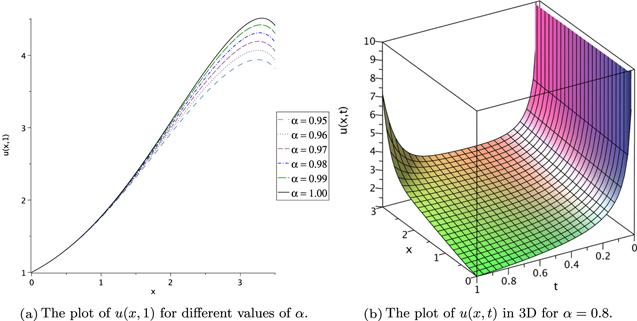
Figure 1. Related plots of the exact solutions of ( |
3.2. Non-classical symmetries
In this case for ξ = 1 and τ = 0 we have31 ) into equation (31 ) yields32 ) is19 ) is as follows:
$\begin{eqnarray}{X}_{3}=x\displaystyle \frac{\partial }{\partial x}+u\displaystyle \frac{\partial }{\partial u},\end{eqnarray}$
and the invariant solution according to this vector field is $\begin{eqnarray}u(x,t)={xf}(t).\end{eqnarray}$
Substituting ( $\begin{eqnarray}\displaystyle \frac{{\partial }^{\alpha }}{\partial {t}^{\alpha }}f(t)+{\beta }_{1}f{\left(t\right)}^{2}=0,\end{eqnarray}$
and therefore, the solution of ( $\begin{eqnarray}f(t)=-\displaystyle \frac{{\rm{\Gamma }}(1-\alpha )}{{\beta }_{1}{\rm{\Gamma }}(1-2\alpha )}{t}^{-\alpha },\end{eqnarray}$
so the exact solution of ( $\begin{eqnarray}u(x,t)=-\displaystyle \frac{{\rm{\Gamma }}(1-\alpha )}{{\beta }_{1}{\rm{\Gamma }}(1-2\alpha )}{{xt}}^{-\alpha }.\end{eqnarray}$
Figure 2 shows the plot of u(x, t) for β1 = β2 = 1 and α = 0.75 in 3D.
Figure 2. Related plot of the exact solution of ( |
For ξ = 1, $\tau \ne 0$ and τu = 0 we have the following vector fields:19 ) can be reduced to the following fractional ODE:
$\begin{eqnarray}\begin{array}{rcl}{X}_{4} & = & (\alpha x+\mu )\displaystyle \frac{\partial }{\partial x}+3t\displaystyle \frac{\partial }{\partial t}-2\alpha u\displaystyle \frac{\partial }{\partial u},\\ {X}_{5} & = & \displaystyle \frac{\partial }{\partial x}+\lambda \displaystyle \frac{\partial }{\partial t}.\end{array}\end{eqnarray}$
By the infinitesimal generator X4, we obtain $\begin{eqnarray}u(x,t)={t}^{\tfrac{-2\alpha }{3}}f(\zeta ),\zeta =\displaystyle \frac{(\alpha x+\mu )}{\alpha }{t}^{\tfrac{-\alpha }{3}},\end{eqnarray}$
and then, equation ( $\begin{eqnarray}\left({{ \mathcal P }}_{\displaystyle \frac{3}{\alpha }}^{1-\tfrac{5\alpha }{3},\alpha }f\right)(\zeta )+{\beta }_{1}f(\zeta )f^{\prime} (\zeta )+{\beta }_{2}f\prime\prime\prime (\zeta )=0,\end{eqnarray}$
so in the same manner used for the infinitesimal generator X2, we have the following exact solution: $\begin{eqnarray}u(x,t)={t}^{\tfrac{-2\alpha }{3}}\sum _{n=0}^{\infty }{a}_{n}{\left(\displaystyle \frac{\alpha x+\mu }{\alpha }{t}^{\tfrac{-\alpha }{3}}\right)}^{n},\end{eqnarray}$
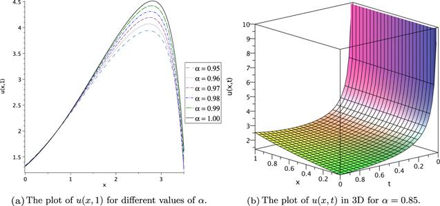
where μ is a constant.In order to illustrate the related plots of the computed exact solution (38 ), we truncate its series with N = 24. Figure 3 shows the plots of u(x, t) for a0 = 1, a1 = 0.5, a2 = 0.25, μ = 0.5 and β1 = β2 = 1. Figure 3 (a) shows the convergence properties of the obtained exact solutions to the exact solution of the integer-order KdV equation when α approaches 1.
Figure 3. Related plots of the exact solutions of ( |
The invariant solution of the infinitesimal generator X519 ) to the time-fractional ODE
$\begin{eqnarray}u(x,t)=f(\zeta ),\zeta =x-\lambda t\end{eqnarray}$
can reduce the equation ( $\begin{eqnarray}{\left(-1\right)}^{\alpha }\frac{{\partial }^{\alpha }}{\partial {\zeta }^{\alpha }}f(\zeta )+{\beta }_{1}f(\zeta )f^{\prime} (\zeta )+{\beta }_{2}f\prime\prime\prime (\zeta )=0,\end{eqnarray}$
and it is not easy to find the exact solution of this equation.4. Conservation laws of the KdV equation
In this part, we turn attention to the nonlinear self-adjointness [45] and new conservation laws (cl) theorem that was first used to construct the cl by Ibragimov in [46]. This theorem uses the LS to find conserved vectors. Here we intend to construct cl for (19 ) according to this method. The cl for equation (19 ) is given by19 ) is given by
$\begin{eqnarray}{D}_{t}{{ \mathcal T }}_{i}^{t}+{D}_{x}{{ \mathcal T }}_{i}^{x}=0,\end{eqnarray}$
where ${{ \mathcal T }}_{i}^{t}={{ \mathcal T }}_{i}^{t}(t,x,u,...)$, ${{ \mathcal T }}_{i}^{x}={{ \mathcal T }}_{i}^{x}(t,x,u,...)$ are the conserved vectors $\begin{eqnarray}\begin{array}{rcl}{{ \mathcal T }}_{i}^{x} & = & \left({}^{u}{{ \mathcal W }}_{i}\displaystyle \frac{\delta { \mathcal H }}{\delta {u}_{x}}+\displaystyle \sum _{k\geqslant 1}{D}_{x}...{D}_{x}({}^{u}{{ \mathcal W }}_{i})\displaystyle \frac{\partial { \mathcal H }}{\partial {u}_{(k+1)x}}\right),\\ {{ \mathcal T }}_{i}^{t} & = & \displaystyle \sum _{k=0}^{n-1}{\left(-1\right)}^{k}{\partial }_{t}^{\alpha -1-k}({}^{u}{{ \mathcal W }}_{i}){D}_{t}^{k}\left(\displaystyle \frac{\partial { \mathcal H }}{\partial ({\partial }_{t}^{\alpha }u)}\right)\\ & & -{\left(-1\right)}^{n}{ \mathcal J }\left({}^{u}{{ \mathcal W }}_{i},{D}_{t}^{n}\left(\displaystyle \frac{\partial { \mathcal H }}{\partial ({\partial }_{t}^{\alpha }u)}\right)\right),\qquad n=[\alpha ]+1,\end{array}\end{eqnarray}$
in which ${}^{u}{{ \mathcal W }}_{i}={\eta }_{i}-{\xi }_{i}{u}_{x}-{\tau }_{i}{u}_{t}$ and the integral ${ \mathcal J }$ is given by $\begin{eqnarray}{ \mathcal J }(h,g)={\int }_{0}^{t}{\int }_{t}^{T}\frac{h(\lambda ,x)g(\mu ,x){\left(\mu -\lambda \right)}^{n-(\alpha +1)}}{{\rm{\Gamma }}(n-\alpha )}{\rm{d}}\lambda {\rm{d}}\mu .\end{eqnarray}$
The formal Lagrangian for ( $\begin{eqnarray}{ \mathcal H }={\rm{\Phi }}(x,t)\left(\displaystyle \frac{{\partial }^{\alpha }u}{\partial {t}^{\alpha }}+{\beta }_{1}{{uu}}_{x}+{\beta }_{2}{u}_{{xxx}}\right),\end{eqnarray}$
where ${\rm{\Phi }}(x,t)={\rm{\Psi }}(x,t,u)$ is a new dependent variable and the adjoint equations of the fractional KdV equation can be specified as follows: $\begin{eqnarray}{{ \mathcal F }}^{* }\equiv \displaystyle \frac{\delta { \mathcal H }}{\delta u}=0,\end{eqnarray}$
where the Euler–Lagrange operators are given by $\begin{eqnarray*}\displaystyle \frac{\delta }{\delta u}=\displaystyle \frac{\partial }{\partial u}+{\left({\partial }_{t}^{\alpha }\right)}^{* }\displaystyle \frac{\partial }{\partial ({\partial }_{t}^{\alpha }u)}+\sum _{k\geqslant 1}{\left(-1\right)}^{k}{D}_{x}...{D}_{x}\displaystyle \frac{\partial }{\partial {u}_{{kx}}},\end{eqnarray*}$
where ${\left({\partial }_{t}^{\alpha }\right)}^{* }$ denotes the adjoint operator for ${\partial }_{t}^{\alpha }$. According to the RL fractional differential operator $\begin{eqnarray*}\begin{array}{rcc}{\left({\partial }_{t}^{\alpha }\right)}^{* } & = & {\left(-1\right)}^{n}{{ \mathcal I }}_{T}^{n-\alpha }({\partial }_{t}^{n})={\left({\partial }_{T}^{\alpha }\right)}_{t}^{{ \mathcal C }},\\ {{ \mathcal I }}_{T}^{n-\alpha }h(t,x) & = & {\int }_{t}^{T}\frac{h(\tau ,x){\left(\tau -t\right)}^{n-(1+\alpha )}}{{\rm{\Gamma }}(n-\alpha )}{\rm{d}}\tau ,\\ n & = & [\alpha ]+1,\end{array}\end{eqnarray*}$
where ${\left({\partial }_{T}^{\alpha }\right)}_{t}^{{ \mathcal C }}$ is the operator of the right-sided Caputo derivative.If we have the following relation for the time-fractional nonlinear equation (44 ), then we can say that equation (19 ) is self-adjoint:46 ) as follows:
$\begin{eqnarray}{{ \mathcal F }}^{* }\equiv \displaystyle \frac{\delta { \mathcal H }}{\delta u}=\mu F,\end{eqnarray}$
where μ remains to be determined. Thus, we can write the nonlinear self-adjoint condition ( $\begin{eqnarray*}\mu =0,\qquad {\rm{\Psi }}(x,t,u)=A,\qquad A\in {\mathbb{R}}.\end{eqnarray*}$
Hence, if we suppose A = 1, then $\begin{eqnarray}{ \mathcal H }=\displaystyle \frac{{\partial }^{\alpha }u}{\partial {t}^{\alpha }}+{\beta }_{1}{{uu}}_{x}+{\beta }_{2}{u}_{{xxx}}.\end{eqnarray}$
According to the above analysis and Lie symmetry generator, we consider the conserved vectors for classical and nonclassical generators of the time-fractional far field KdV equation. We have the following cases for classical generators:Case 1: Here for the first classical generator X1, the respective Lie characteristic function is48 ) into (42 ) yields the conserved vector as follows:
$\begin{eqnarray}{}^{u}{{ \mathcal W }}_{1}=-{u}_{x}.\end{eqnarray}$
Substituting ( $\begin{eqnarray*}\begin{array}{rcl}{{ \mathcal T }}_{1}^{x} & = & {}^{u}{{ \mathcal W }}_{1}\left(\displaystyle \frac{\partial { \mathcal H }}{\partial {u}_{x}}-{D}_{x}\displaystyle \frac{\partial { \mathcal H }}{\partial {u}_{{xx}}}+{D}_{x}^{2}\displaystyle \frac{\partial { \mathcal H }}{\partial {u}_{{xxx}}}\right)\\ & & +{D}_{x}({}^{u}{{ \mathcal W }}_{1})\displaystyle \frac{\partial { \mathcal H }}{\partial {u}_{{xx}}}+{D}_{x}^{2}({}^{u}{{ \mathcal W }}_{1})\displaystyle \frac{\partial { \mathcal H }}{\partial {u}_{{xxx}}},\\ {{ \mathcal T }}_{1}^{t} & = & {{ \mathcal I }}^{1-\alpha }({}^{u}{{ \mathcal W }}_{1}){\rm{\Psi }}+{ \mathcal J }\left({}^{u}{{ \mathcal W }}_{1},{{\rm{\Psi }}}_{t}\right),\end{array}\end{eqnarray*}$
then $\begin{eqnarray*}\begin{array}{rcl}{{ \mathcal T }}_{1}^{x} & = & -{u}_{x}({\beta }_{1}u+{\beta }_{2})+{\beta }_{2}{u}_{{xx}}+{\beta }_{2}{u}_{{xxx}}\\ {{ \mathcal T }}_{1}^{t} & = & -{{ \mathcal I }}^{1-\alpha }{u}_{x}{\rm{\Psi }}+{ \mathcal J }\left(-{u}_{x},{{\rm{\Psi }}}_{t}\right).\end{array}\end{eqnarray*}$
Case 2: For the generator ${X}_{2}=\alpha x\displaystyle \frac{\partial }{\partial x}\,+3t\displaystyle \frac{\partial }{\partial t}\,-2\alpha u\displaystyle \frac{\partial }{\partial u}$, the respective Lie characteristic function is obtained by49 ) into (42 ) yields
$\begin{eqnarray}{}^{u}{{ \mathcal W }}_{2}=-2\alpha u-\alpha {{xu}}_{x}-3{{tu}}_{t}.\end{eqnarray}$
Substituting ( $\begin{eqnarray*}\begin{array}{rcl}{{ \mathcal T }}_{2}^{x} & = & -\left({\beta }_{1}u+{\beta }_{2}\right)\left(2\alpha u+\alpha {{xu}}_{x}+3{{tu}}_{t}\right)\\ & & +{\beta }_{2}\left(3\alpha {u}_{x}+\alpha {{xu}}_{{xx}}+3{{tu}}_{{xt}}\right)\\ & & -{\beta }_{2}\left(4\alpha {u}_{{xx}}+\alpha {{xu}}_{{xxx}}+3{{tu}}_{{xxt}}\right),\\ {{ \mathcal T }}_{2}^{t} & = & -{{ \mathcal I }}^{1-\alpha }(2\alpha u+\alpha {{xu}}_{x}+3{{tu}}_{t}).\end{array}\end{eqnarray*}$
For nonclassical generators:Case 3: For ξ = 1 and τ = 0 we have ${X}_{3}=x\displaystyle \frac{\partial }{\partial x}\,+u\displaystyle \frac{\partial }{\partial u}$, and the respective Lie characteristic function is obtained by50 ) into (42 ) yields the conserved vector as follows:
$\begin{eqnarray}{}^{u}{{ \mathcal W }}_{3}=u-{{xu}}_{x}.\end{eqnarray}$
Hence, substituting ( $\begin{eqnarray*}\begin{array}{rcl}{{ \mathcal T }}_{3}^{x} & = & \left({\beta }_{1}u+{\beta }_{2}\right)\left(u-{{xu}}_{x}\right)+{\beta }_{2}{{xu}}_{x}-{\beta }_{2}\left({u}_{{xx}}+{{xu}}_{{xxx}}\right)\\ {{ \mathcal T }}_{3}^{t} & = & {{ \mathcal I }}^{1-\alpha }(u-{{xu}}_{x}).\end{array}\end{eqnarray*}$
Case 4: For ξ = 1 and $\tau \ne 0$, we have ${X}_{4}=(\alpha x\,+\mu )\displaystyle \frac{\partial }{\partial x}+3t\displaystyle \frac{\partial }{\partial t}-2\alpha u\displaystyle \frac{\partial }{\partial u}$. The respective Lie characteristic function is obtained by
$\begin{eqnarray}{}^{u}{{ \mathcal W }}_{4}=-2\alpha u-(\alpha x+\mu ){u}_{x}-3{{tu}}_{t}.\end{eqnarray}$
The corresponding conserved vectors are $\begin{eqnarray*}\begin{array}{rcl}{{ \mathcal T }}_{4}^{x} & = & -\left({\beta }_{1}u+{\beta }_{2}\right)\left(2\alpha u+\left(\alpha x+\mu \right){u}_{x}+3{{tu}}_{t}\right)\\ & & +{\beta }_{2}\left(3\alpha {u}_{x}+(\alpha x+\mu ){u}_{{xx}}+3{{tu}}_{{xt}}\right)\\ & & -{\beta }_{2}\left(4\alpha {u}_{{xx}}+(\alpha x+\mu ){u}_{{xxx}}+3{{tu}}_{{xxt}}\right),\\ {{ \mathcal T }}_{4}^{t} & = & -{{ \mathcal I }}^{1-\alpha }(2\alpha u+(\alpha x+\mu ){u}_{x}+3{{tu}}_{t}).\end{array}\end{eqnarray*}$
Case 5: The respective Lie characteristic function for ${X}_{5}=\displaystyle \frac{\partial }{\partial x}+\lambda \displaystyle \frac{\partial }{\partial t}$ is obtained by
$\begin{eqnarray}{}^{u}{{ \mathcal W }}_{5}=-{u}_{x}-\lambda {u}_{t}.\end{eqnarray}$
The corresponding conserved vectors are $\begin{eqnarray*}\begin{array}{rcl}{{ \mathcal T }}_{5}^{x} & = & -\left({\beta }_{1}u+{\beta }_{2}\right)\left({u}_{x}+\lambda {u}_{t}\right)\\ & & +{\beta }_{2}\left({u}_{{xx}}+\lambda {u}_{{xt}}\right)-{\beta }_{2}\left({u}_{{xxx}}+\lambda {u}_{{xxt}}\right),\\ {{ \mathcal T }}_{5}^{t} & = & -{{ \mathcal I }}^{1-\alpha }({u}_{x}+\lambda {u}_{t}).\end{array}\end{eqnarray*}$
5. Conclusion
In this work, we mainly study the classical Lie symmetry, nonclassical Lie symmetry and conservation laws of the nonlinear time-fractional KdV equation. We use the symmetry of the Lie group analysis for the nonlinear time-fractional far field KdV equation and employ classical and nonclassical Lie symmetry to acquire similarity reductions of this equation according to the obtained vector fields and the corresponding invariant solutions. We also find the related exact solutions by some methods like the power series method for the derived generators. From figures 1 and 3, one may find that our obtained solutions in both the classical and nonclassical cases have convergence behavior. Finally, according to the LS generators acquired, we construct conservation laws for related classical and nonclassical vector fields of the mentioned equation. From these findings, we conclude that the presented method might become a promising one in finding the analytical solutions of different kinds of fractional partial differential equations.