


1. Introduction
2. DT for the time-reversal nonlocal nonlinear Schödinger equation
The DT (
The proof of this theorem is equivalent to verify the following two equations:
Defining
Now we proceed to prove the symmetric properties of ${{\boldsymbol{U}}}^{[1]}$ and ${{\boldsymbol{V}}}^{[1]}$. Since ${{\boldsymbol{\Psi }}}^{\dagger }(x,-t;-\lambda ){\boldsymbol{C}}{\boldsymbol{\Psi }}(x,t;\lambda ){\boldsymbol{C}}={\mathbb{I}}$, then
If we have N different solutions to system (
The recursive DTs between matrix functions are given as
3. Bounded multi-solitons solutions and their asymptotic analysis
3.1. The dynamics for the single-soliton solution
3.1.1. Singularity
3.1.2. Boundedness
3.1.3. Oscillation effect

Figure 1. (a) By choosing the parameters ${a}_{1}=10$, ${b}_{1}=\tfrac{1}{2}$, c = 1, $\sigma =-1$, we obtain an unbounded non-singular single-soliton solution. (b) The corresponding sectional view of the single-soliton solution in (a) and its lower envelope. (c) By setting ${a}_{1}=0$, ${b}_{1}=1$, $c=1+{\rm{i}}$, $\sigma =-1$, we obtain a bounded non-singular single-soliton solution. |
The distance between the two abscissa corresponding to 1/2 of the maximum of the lower envelope is defined as the width of the soliton solution oscillation.
Choosing the parameters appropriately we have drawn graphs of unbounded single-soliton solutions and bounded single-soliton solutions. And from figure 1(a), we can see the single-soliton emerging the effect of periodic oscillation. Also, we provide the sectional view of the single-soliton solution and the lower envelope.
3.2. The non-singular symmetric multi-soliton solution
[40]
From equation (
From theorem
For a 2n-soliton solution, if the parameters satisfy
Firstly, we verify that ${\boldsymbol{M}}$ is non-degenerate. By theorem
By theorem
In the above proposition, we give a sufficient condition for the $2n$-soliton solution with pair parameters. Actually, for the case ${\lambda }_{i}\in {\rm{i}}{\mathbb{R}}$, we can also obtain the similar result in a similar way. In this case, what we obtain are also the bounded non-singular soliton solutions.
3.3. Asymptotic analysis for the multi-soliton solution
Choosing the parameters as ${a}_{1}=1,{b}_{1}=1,\sigma =-1$, we construct the asymptotic form of the two-soliton solution. Due to the symmetry of the solution with respect to the time variable t, here we only show the sectional view when $t\to +\infty $. The results are shown in figure 2.
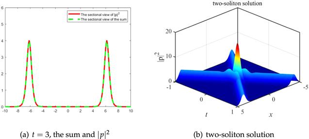
Figure 2. ${a}_{1}=1,{b}_{1}=1$ (a) The red solid lines represent the sectional view of $| {p}^{[2]}{| }^{2}$ when t = 3. The green dotted lines represent the sectional view of the sum of the two decomposed single-soliton solutions with t = 3. It is shown that the sum matches $| {p}^{[2]}{| }^{2}$ very well. (b) two-soliton solution: a1 = 2, b1 = 1, σ = −1. |
For a $2n$-soliton solution ${p}^{[2n]}$, if the selected parameters satisfy the following conditions
We regard two adjacent matrix functions as a pair, and the expression of any pair is given as follows
When $t\to +\infty $, fixed the direction as $x+2{a}_{i}t={\theta }_{2i-1}$, we can deduce that
$|{\tilde{{\boldsymbol{M}}}}_{2i-1}| = $
$\begin{eqnarray*}\begin{array}{rcl} \left|\begin{array}{ccccccc}\displaystyle \frac{1}{2({\lambda }_{i+1}-{\lambda }_{i+1}^{* })} & ... & \displaystyle \frac{1}{2({\lambda }_{n}-{\lambda }_{i+1}^{* })} & \displaystyle \frac{1}{2({\lambda }_{i}-{\lambda }_{i+1}^{* })} & 0 & ... & 0\\ \vdots & & \vdots & \vdots & \vdots & & \vdots \\ \displaystyle \frac{1}{2({\lambda }_{i+1}-{\lambda }_{n}^{* })} & ... & \displaystyle \frac{1}{2({\lambda }_{n}-{\lambda }_{n}^{* })} & \displaystyle \frac{1}{2({\lambda }_{i}-{\lambda }_{n}^{* })} & 0 & ... & 0\\ \displaystyle \frac{1}{2({\lambda }_{i+1}-{\lambda }_{i}^{* })} & ... & \displaystyle \frac{1}{2({\lambda }_{n}-{\lambda }_{i}^{* })} & \displaystyle \frac{1}{2({\lambda }_{i}-{\lambda }_{i}^{* })} & \displaystyle \frac{{{\rm{e}}}^{{\eta }_{i}^{* }(x,t)}}{2({\lambda }_{1}-{\lambda }_{i}^{* })} & ... & \displaystyle \frac{{{\rm{e}}}^{{\eta }_{i}^{* }(x,t)}}{2(-{\lambda }_{n}^{* }-{\lambda }_{i}^{* })}\\ 0 & ... & 0 & 0 & \displaystyle \frac{1}{2({\lambda }_{1}+{\lambda }_{1})} & ... & \displaystyle \frac{1}{2(-{\lambda }_{n}^{* }+{\lambda }_{1})}\\ \vdots & & \vdots & \vdots & \vdots & & \vdots \\ 0 & ... & 0 & 0 & \displaystyle \frac{1}{2({\lambda }_{1}-{\lambda }_{i-1}^{* })} & ... & \displaystyle \frac{1}{2(-{\lambda }_{n}^{* }-{\lambda }_{i-1}^{* })}\end{array}\right| \end{array}\end{eqnarray*}$
$\begin{eqnarray*}\begin{array}{rcl} & + & \left|\begin{array}{ccccccc}\displaystyle \frac{1}{2({\lambda }_{i+1}-{\lambda }_{i+1}^{* })} & ... & \displaystyle \frac{1}{2({\lambda }_{n}-{\lambda }_{i+1}^{* })} & 0 & 0 & ... & 0\\ \vdots & & \vdots & \vdots & \vdots & & \vdots \\ \displaystyle \frac{1}{2({\lambda }_{i+1}-{\lambda }_{n}^{* })} & ... & \displaystyle \frac{1}{2({\lambda }_{n}-{\lambda }_{n}^{* })} & 0 & 0 & ... & 0\\ \displaystyle \frac{1}{2({\lambda }_{i+1}-{\lambda }_{i}^{* })} & ... & \displaystyle \frac{1}{2({\lambda }_{n}-{\lambda }_{i}^{* })} & \displaystyle \frac{{{\rm{e}}}^{2({\eta }_{i}(x,t)+{\eta }_{i}^{* }(x,t))}}{2({\lambda }_{i}-{\lambda }_{i}^{* })} & \displaystyle \frac{{{\rm{e}}}^{{\eta }_{i}^{* }(x,t)}}{2({\lambda }_{1}-{\lambda }_{i}^{* })} & ... & \displaystyle \frac{{{\rm{e}}}^{{\eta }_{i}^{* }(x,t)}}{2(-{\lambda }_{n}^{* }-{\lambda }_{i}^{* })}\\ 0 & ... & 0 & \displaystyle \frac{{{\rm{e}}}^{2{\eta }_{i}(x,t)}}{2({\lambda }_{i}+{\lambda }_{1})} & \displaystyle \frac{1}{2({\lambda }_{1}+{\lambda }_{1})} & ... & \displaystyle \frac{1}{2(-{\lambda }_{n}^{* }+{\lambda }_{1})}\\ \vdots & & \vdots & \vdots & \vdots & & \vdots \\ 0 & ... & 0 & \displaystyle \frac{{{\rm{e}}}^{2{\eta }_{i}(x,t)}}{2({\lambda }_{i}-{\lambda }_{i-1}^{* })} & \displaystyle \frac{1}{2({\lambda }_{1}-{\lambda }_{i-1}^{* })} & ... & \displaystyle \frac{1}{2(-{\lambda }_{n}^{* }-{\lambda }_{i-1}^{* })}\end{array}\right| & & \\ & = & \displaystyle \frac{1}{{2}^{2n}}\left[{C}_{1}{C}_{2}+{C}_{3}{C}_{4}{{\rm{e}}}^{2({\eta }_{i}(x,t)+{\eta }_{i}^{* }(x,t))}\right]\\ & = & \displaystyle \frac{1}{{2}^{2n}}\left[\displaystyle \frac{1}{{\lambda }_{i}-{\lambda }_{i}^{* }}{C}_{2}{C}_{3}\left({\gamma }_{2i-\mathrm{1,1}}+{\gamma }_{2i-\mathrm{1,2}}{{\rm{e}}}^{2({\eta }_{i}(x,t)+{\eta }_{i}^{* }(x,t))}\right)\right],\end{array}\end{eqnarray*}$
where
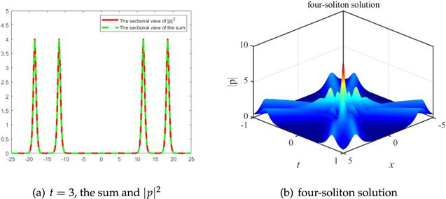
Choosing the parameters as ${a}_{1}=2,{b}_{1}=1,{a}_{2}=3,{b}_{2}=1,\sigma =-1$, we construct the asymptotic form of a four-soliton solution to test the result of theorem
Figure 3. ${a}_{1}=1,{b}_{1}=1,{a}_{2}=3,{b}_{2}=1$ (a) The red solid lines represent the sectional view of $| {p}^{[4]}{| }^{2}$ when t = 3. The green dotted lines represent the sectional view of the sum of the four decomposed single-soliton solutions with t = 3. It is shown that the sum matches $| {p}^{[4]}{| }^{2}$ very well. (b) four-soliton solution: ${a}_{1}=2,{b}_{1}=1,{a}_{2}=3,{b}_{2}=1,\sigma =-1$. |
For a $(2n+1)$-soliton solution, if the added parameter ${\lambda }_{2n+1}$ satisfies ${\mathfrak{R}}({\lambda }_{2n+1})=0$, then the result still holds.
For the $\sigma =1$, by setting the solution parameter ci of each matrix function ${{\boldsymbol{\psi }}}_{i}(x,t)$ as ${\rm{i}}$, we can not only ensure the non-singularity of the soliton solution, but also obtain the same ${\bf{M}}$ matrix as in the case of $\sigma =-1$. So it can be similarly verified that
Compared to the classical NLSE, the asymptotic decomposition of the multi-soliton solutions of the nNLS equation under study is only applicable to the symmetric soliton solutions. In addition, the classical NLSE has not only the asymptotic expression of the square of the modulus of the solution, but also other forms of asymptotic expressions of the solution. What is more, there is no phase shift character in our asymptotic analysis, but in general it does exist in classical NLSE.