The (3 + 1)-dimensional Zakharov–Kuznetsov (ZK) and the new extended quantum ZK equations are functional to decipher the dense quantum plasma, ion-acoustic waves, electron thermal energy, ion plasma, quantum acoustic waves, and quantum Langmuir waves. The enhanced modified simple equation (EMSE) method is a substantial approach to determine competent solutions and in this article, we have constructed standard, illustrative, rich structured and further comprehensive soliton solutions via this method. The solutions are ascertained as the integration of exponential, hyperbolic, trigonometric and rational functions and formulate the bright solitons, periodic, compacton, bell-shape, parabolic shape, singular periodic, plane shape and some new type of solitons. It is worth noting that the wave profile varies as the physical and subsidiary parameters change. The standard and advanced soliton solutions may be useful to assist in describing the physical phenomena previously mentioned. To open out the inward structure of the tangible incidents, we have portrayed the three-dimensional, contour plot, and two-dimensional graphs for different parametric values. The attained results demonstrate the EMSE technique for extracting soliton solutions to nonlinear evolution equations is efficient, compatible and reliable in nonlinear science and engineering.
M Ali Akbar, Md Abdul Kayum, M S Osman. Bright, periodic, compacton and bell-shape soliton solutions of the extended QZK and (3 + 1)-dimensional ZK equations[J]. Communications in Theoretical Physics, 2021, 73(10): 105003. DOI: 10.1088/1572-9494/ac1a6c
1. Introduction
Nonlinear evolution equations (NLEEs) play a very important role in describing many physical features, particularly in quantum acoustic waves, quantum Langmuir waves, dense quantum plasma, ion-acoustic waves, electron thermal energy, ion plasma, solid state physics, optical fibers, chemical physics, chaos theory, mathematical physics, astrophysics, biophysics, nuclear physics, fluid mechanics, engineering problems [1, 2] etc. Nonlinear soliton solutions of these NLEEs play a fundamental role in unraveling the dynamics and describing the facts. Thus, different methods are used to search soliton solutions to these NLEEs. Some of them are the extended simple equation technique [3], the generalized Kudryashov technique [4], the first-integral technique [5], the new auxiliary equation technique [6], the Bernoulli sub-equation function technique [7, 8], the Riccati–Bernoulli sub-ODE method [9–11], the sine-Gordon expansion technique [12, 13], the sine–cosine technique [14], the generalized unified technique [15], the modified Khater method [16], the tanh–coth method [17], He's variational principle [18, 19], the B$\ddot{{\rm{a}}}$cklund transformation method [20], the unified Riccati equation expansion method [21], the extended Kudryashov method [22], the improved $(G^{\prime} /G)$-expansion method [23], the functional variable method [24], the exp-expansion technique [25], the improved $F$-expansion technique [26], the MSE technique [27–30], the enhanced MSE method [31], the Jacobi elliptic functions method [32–35], and other different techniques [36–40].
In various fields of physics, applied mathematics, and engineering, the Zakharov–Kuznetsov (ZK) equation is used. The new extended quantum ZK (QZK) and the (3 + 1)-dimensional ZK equations were derived for finite but small amplitude ion-acoustic waves in a quantum magneto-plasma by using the reductive perturbation theory and the quantum hydrodynamical model [41]. In this study, we consider the enhanced MSE technique to search bright solitons, periodic, compacton, bell-shape, parabolic, singular periodic and other general soliton solutions of the (3 + 1)-dimensional ZK equation and the new extended quantum QZK equation [42]. The ZK equation is one of the two canonical two-dimensional extensions of the Korteweg–de Vries equation, which was initially developed in two dimensions for weakly nonlinear ion-acoustic waves in strongly magnetized lossless plasma. The new extended QZK equation [43] is:
where $v(x,y,t)$ represents the electrostatic wave potential with the temporal variable $t$ and spatial variables $x,$ $y$ and $\alpha ,\beta ,\gamma $ are all constants. The coefficients of $\beta $ and $\gamma $ describe the multi-dimensional dispersion terms, the coefficient of $\alpha $ is the nonlinear term, and ${v}_{t}$ is the evolution with respect to time.
In the subsequent, we consider the (3 + 1)-dimensional ZK [44]:
where α is the nonlinear coefficient and $\beta ,$ $\gamma ,$ $\delta $ are the dispersion coefficients. In [44], the ZK equation was derived by putting in use the reductive perturbation technique and the quantum hydrodynamic model and some periodic, explosive, and solitary wave solutions are obtained with the help of the extended Conte's truncation technique.
The exact solutions and symmetry reductions to the extended QZK equation have been derived by Lie symmetry analysis in [45]. In [46], the optimal system and conservation law were used for further investigation of the extended QZK equation. To obtain the exact travelling wave solutions to the extended QZK equation, El-Ganaini and Akbar [47] contrive the modified simplest equation technique, the extended simplest equation technique, and the simplest equation technique. Baskonus et al [48] extracted hyperbolic and complex function solutions of the extended QZK equation by using the sine-Gordon expansion technique. Raza et al [49] used the trial equation method to search soliton and periodic solutions of equation (1).
The multiple soliton solutions and new exact solitary wave solutions of (2) were attained by means of the Hirota's bilinear technique and the auxiliary equation method in [50]. Ebadi et al [51] used the adapted $F$-expansion technique, exp-function technique, and the $(G^{\prime} /G)$-expansion technique to find exact travelling wave solutions. Bhrawy et al [52] introduced the extended $F$-expansion technique for finding the complexiton solutions, singular soliton, non-topological, and topological solutions. In [53], the authors applied the extended generalized $(G^{\prime} /G)$-expansion technique to determine new exact solutions of (2). Lu et al [54] introduced the modified extended direct algebraic method to extract the elliptic function solutions, soliton and new exact solitary wave solutions of (2). New types of travelling wave solutions of (2) were attained by applying the generalized $(G^{\prime} /G)$-expansion technique and the improved $\tan (\phi /2)$-expansion technique in [55]. Zayed et al [56] applied the $(G^{\prime} /G,\,1/G)$-expansion method to extract further exact solutions of (2). Recently, Vinita and Ray [57] used the Lie symmetry analysis to study the equation (2) and new exact solitary wave solutions are attained and also derived the conservation laws to the QZK equation.
The enhanced modified simple equation (EMSE) method is recently developed a significant approach to determining competent solutions that is effective, compatible, and reliable to extract soliton solutions to NLEEs. This method have been used to examine the (1 + 1)-dimensional Burgers–Fisher equation with variable coefficients, the (2 + 1)-dimensional ZK equation with variable coefficient, the FitzHugh–Nagumo equation, the Burgers–Huxley equation [58], the modified Volterra equations, the Burger–Fisher equation [59], the Phi-4 equation [60], Chafee–Infante equation [61], the Gardner equation and the modified Benjamin–Bona–Mahony equation [62]. The (3 + 1)-dimensional ZK and the new extended QZK equations are important mathematical models to decipher ion-acoustic waves, quantum acoustic waves, quantum Langmuir waves, etc. To the optimal of our cognition and based on the analysis of the documents reachable in the literature obtained, the formerly introduced equations have not been investigated by the EMSE technique earlier. Thus, supported by the earlier studies, the aim of this article is to ascertain standard, realistic and far-reaching compatible solutions to these equations through the EMSE method. The feature of the solutions is that they extract bright solitons, periodic, compacton, bell-shape, parabolic shape, singular periodic and other solitons for certain values of the associated parameters.
The remaining of the article is sorted out as follows: the explanation of the enhanced MSE technique is given in section 2. In section 3, we use technique to search the advanced and wide-spectral soliton solutions. Some of the important graphical depictions of the solutions obtained are given in section 4. Finally in the last section, the conclusion is given.
2. The EMSE technique
In this section, we concisely explain the EMSE technique [58–62]. Let us consider a general NLEE in the subsequent form:
where $ {\mathcal L} $ is a polynomial with respect to the wave function $v(x,y,z,t)$ in which the highest order derivatives and nonlinear terms are involved. The following are the basic steps of this technique:
The wave variable $\xi =p\left(t\right)x$ $+q\left(t\right)y$ $+r\left(t\right)z+s(t),$ where $v\left(x,y,z,t\right)=V(\xi )$ remodels equation (3) into a nonlinear differential equation in the follow way:
where $V=V(\xi ),$ dot specifies the differentiation related to time $t,$ and prime ($^{\prime} $) specifies the differentiation with respect to $\xi .$
The solution of the reduced equation (4), in agreement with the EMSE method can be put into the form:
where ${a}_{0}\left(t\right),$ ${a}_{1}\left(t\right),$ ${a}_{2}\left(t\right),$…,${a}_{N}(t)$ are the unknown function of ‘$t$' to be evaluated, such that ${a}_{N}(t)\ne 0,$ and $\psi ^{\prime} \left(\xi \right)\ne 0.$ The outstanding feature of this approach is that, instead of constants, the coefficients of $\psi {\left(\xi \right)}^{-i}$ are the function of $t,$ and $\psi \left(\xi \right)$ is an unknown function or not a solution of any well-known equation.
The balancing theory between the nonlinear and linear terms appearing in equation (4), results the balance number $N$ arise in solution (5).
Using the solution (5) and its necessary derivatives into equation (4), together with the balance number $N,$ yield a polynomial of $\psi {\left(\xi \right)}^{-i},$ where $i=1,$ $2,$ $3,$…,$N.$ Collecting all the terms of same power and equating them to zero, it is attained a system of differential and algebraic equations, can be estimated to find ${a}_{0},$ ${a}_{i},$ $p,$ $q,$ $r,$ $s$ and $\psi (\xi ).$ Thus, we can establish inclusive, fresh and standard soliton solutions of (3) by substituting the above values into the solution (5).
3. Solutions analysis
In this section, bright solitons, periodic, compacton, parabolic, bell-shape, singular periodic and other types of soliton solutions of the (3 + 1)-dimensional ZK and the new extended QZK equations are established via the enhanced MSE technique.
3.1. The new extended QZK equation
In this section, we derive the general solitary wave solution in terms of hyperbolic function, trigonometric function, exponential function and rational function of the new extended QZK equation using the enhance MSE technique. The wave transformation
Inserting solution (9) and its necessary derivatives into equation (8); equating all the coefficients of ${\psi }^{-i},\,x{\psi }^{-i},\,y{\psi }^{-i},$ $i=0,$ $1,$ $2,$ $3,$ $4,$ and setting them to zero, we attain the algebraic and differential equations as follows:
where ${c}_{1},\,{c}_{2}$ are constants of integration and $K\,=\tfrac{{a}_{1}\left(2{h}^{3}\beta +2{k}^{3}\beta +2{h}^{2}k\gamma +2h{k}^{2}\gamma +h\alpha {a}_{2}\right)}{10\left(h+k\right)\left({h}^{2}\beta -hk\beta +{k}^{2}\beta +hk\gamma \right){a}_{2}}.$
The following cases should now be discussed:
When ${a}_{0}=0.$
Inserting the values of $\psi (\xi ),$ ${a}_{2}(t)$ and ${a}_{0}(t)$ into (13), we obtain
Since the values of $p,$ $q,$ ${a}_{0},$ ${a}_{1},$ ${a}_{2}$ and $\psi $ satisfy equation (16), the values of $p,$ $q,$ ${a}_{0},$ ${a}_{1},$ ${a}_{2}$ and $\psi $ are admissible to determine the soliton solutions.
Using the values of ${a}_{0},\,{a}_{1},\,{a}_{2}$ and $\psi (\xi )$ into the solution (9), we ascertain
Moreover, if we assign, ${c}_{1}=\pm G,$ ${c}_{2}=\pm 1$ or ${c}_{1}=\pm 1,$ ${c}_{2}=\pm \tfrac{1}{G},$ we obtain the succeeding hyperbolic function solutions of equation (8)
Alternatively, if we set ${c}_{1}=\pm H,\,{c}_{2}=\pm 1$ or ${c}_{1}=\pm 1,{c}_{2}=\pm \tfrac{1}{H},$ we ascertain the under mentioned soliton solutions
where $G$ is provided in the above. The solutions (28)–(31) and (38)–(41) represent bright, parabolic soliton, bell-shape soliton, singular periodic soliton, and compacton.
3.2. The (3 + 1)-dimensional ZK equation
In this section, relating to exponential function, rational function, hyperbolic function and trigonometric function, we obtain the general solitary wave solution to the (3 + 1)-dimensional ZK equation via the EMSE method. The wave variable
where ${a}_{0},$ ${a}_{1}$ and ${a}_{2}$ are an unknown function of $t,$ and $\psi ^{\prime} \left(\xi \right)\ne 0.$
Putting the values of $V\left(\xi \right)$ and it's twice derivative into (44) and equalizing the coefficients of same power to zero, we attain some algebraic and differential equations as follows:
where ${c}_{3}$ and ${c}_{4}$ are constants of integration and $K^{\prime} \,=\tfrac{{a}_{1}\left(2{n}^{2}\beta +2{l}^{2}\gamma +2{m}^{2}\delta +\alpha {a}_{2}\right)}{10\left({n}^{2}\beta +{l}^{2}\gamma +q{m}^{2}\delta \right){a}_{2}}.$
Solving equations (46) and (59) and putting the values of $p,q,r,$ we attain
Inasmuch as equation (54) is satisfied for the values of $p,$ $q,$ $r,$ ${a}_{0},$ ${a}_{1},$ ${a}_{2}$ and $\psi ,$ these values are acceptable for determining the soliton solutions.
Substituting the values of ${a}_{0},$ ${a}_{1},$ ${a}_{2}$ and $\psi $ into the solution (45), we attain the subsequent exponential function solution
Since ${c}_{3}$ and ${c}_{4}$ are integral constants, their values could be set at random. As a result, we can choose the values of ${c}_{3}$ and ${c}_{4}$ arbitrarily. Therefore, if we choose ${c}_{3}=\pm 5/2$ and ${c}_{4}=\pm 1/2M,$ the solution (62) turns out to be
Again, if we choose ${c}_{3}=\pm M,$ ${c}_{4}=\pm 1$ or ${c}_{3}=\pm 1,$ ${c}_{4}=\pm \tfrac{1}{M},$ we attain the hyperbolic function solutions of equation (44) in the ensuing
The solutions (66)–(69) and (75)–(78) produce the bright, periodic, singular bell-shaped and plane shaped solitons which helps to understand the physical features of the (3 + 1)-dimensional ZK equation.
4. Results and discussion
The symbolic demonstration is very significant to understand the physical context of the solutions obtained for diverse parameter values. Therefore, we have portrayed two and three-dimensional graphics of the completed solutions to the (3 + 1)-dimensional ZK equation and the new extended QZK equation, in this section. To ascertain the physical properties of the earlier described equations, graphical descriptions of some of the solutions obtained by Matlab software are portrayed. Since the arbitrarily function $r(t)$ of the new extended QZK equation and $s(t)$ of the (3 + 1)-dimensional ZK equation exist in the solutions, therefore we may choose their values randomly for each solution. Figures 1–8 show the two and three-dimensional diagrams of the obtained solutions for the new extended QZK equation, and figures 9–16 indicate the two and three-dimensional graphs for the (3 + 1)-dimensional ZK equation. In figures 1–8, the 3D graphs are portrayed at $y=0$ and 2D graphs are depicted at $x=y=0.$ Also, in figures 9–16, the 3D graphs are depicted at $y=z=0$ and the 2D graphs are illustrated at $x=y=z=0.$
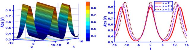
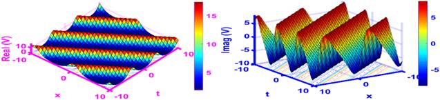
Figure 1. The 3D and 2D graphics for $r\left(t\right)=\lambda t$ of the solution (24) with the parametric values $h=2,\,k=1,\,\alpha =6,\,\beta =2,\,\gamma =2$ and $\lambda =2.$
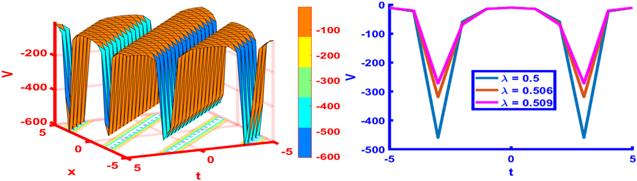
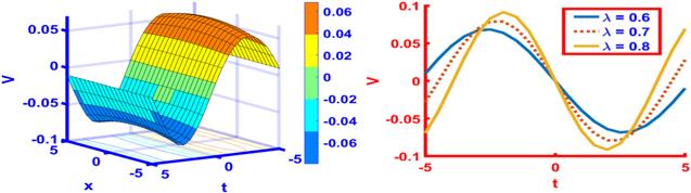
Figure 2. The 3D and 2D graphics for r (t) = λt of the solution (28) with the parametric values $h=0.5,$ $k=0.2,$ $\alpha =0.3,$ $\beta =0.4,$ $\gamma =0.6$ and $\lambda =0.5.$
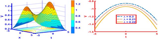
Figure 3. The 3D and 2D graphics for $r\left(t\right)=\,\sinh \left(\lambda t\right)$ of the solution (28) with parametric values $h=0.7,$ $k=-1,$ $\alpha =-1,$ $\beta =2,$ $\gamma =3$ and $\lambda =0.2.$
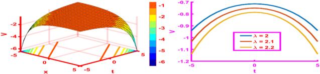
Figure 4. The 3D and 2D graphics for $r\left(t\right)=\lambda t$ of the solution (29) with particular values $h=4,$ $k=4,$ $\alpha =3,$ $\beta =-0.1,$ $\gamma =0.3$ and $\lambda =4.$
Figure 5. The 3D and 2D graphics for $r\left(t\right)=\lambda {\rm{t}}$ of the solution (30) with the particular values $h=2.8,$ $k=3,$ $\alpha =3,$ $\beta =2,$ $\gamma =1.9$ and $\lambda =2.$
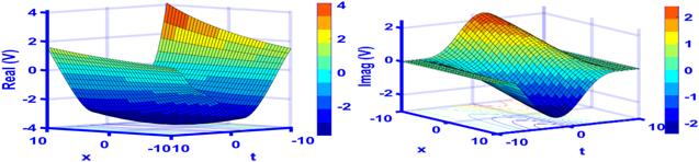
Figure 6. The 3D graphics for $r\left(t\right)=\lambda {\rm{t}}$ of the solution (34) with the particular values $h=0.7,$ $k=1,$ $\alpha =0.4,$ $\beta =0.4,$ $\gamma =0.6$ and $\lambda =-1.$
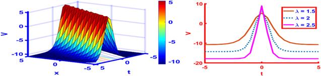
Figure 7. The 3D and 2D graphics for $r\left(t\right)=\lambda {\rm{t}}$ of the solution (38) with the particular values $h=0.7,$ $k=1,$ $\alpha =0.4,$ $\beta =0.4,$ $\gamma =0.6$ and $\lambda =1.5.$
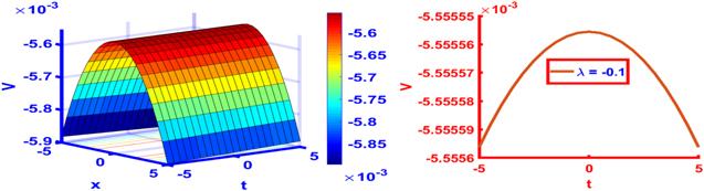
Figure 8. The 3D and 2D graphics for $r\left(t\right)=\lambda {\rm{t}}$ of the particular solution (40) with the parametric values $h=9,$ $k=-0.8,$ $\alpha =2,$ $\beta =4,$ $\gamma =6$ and $\lambda =-0.1.$
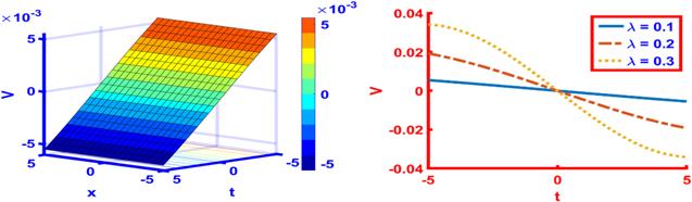
Figure 9. The 3D graphics for $s\left(t\right)=\,\sin \left(\lambda {\rm{t}}\right)$ of the solution (63) with the parametric values $l=-0.1,$ $m=0.3,$ $n=1,$ $\delta =0.8,$ $\gamma =0.6,$ $\beta =0.9,$ $\alpha =0.4$ and $\lambda =0.2.$
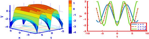
Figure 10. The 3D and 2D graphics for $s\left(t\right)=\,\sin \left(\lambda {\rm{t}}\right)$ of the general solution (66) with the parametric values $l=0.6,$ $m=0.8,$ $n=1,$ $\alpha =2,$ $\beta =4,$ $\gamma =2,$ $\delta =1$ and λ = 1.
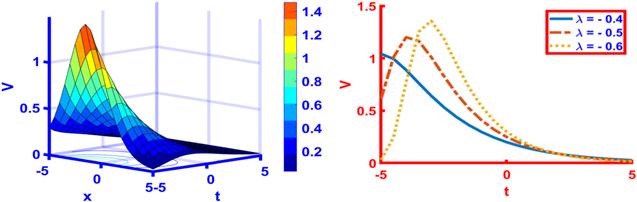
Figure 11. The 3D and 2D graphics for $s\left(t\right)={{\rm{e}}}^{\lambda {\rm{t}}}$ of the solution (66) with the particular values $l=5,$ $m=0.5,$ $n=2,$ $\alpha =3,$ $\beta =1,$ $\gamma =2,$ $\delta =2$ and $\lambda =-0.4.$
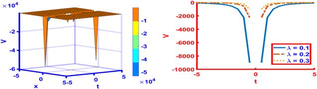
Figure 12. The 3D and 2D graphics for $s\left(t\right)=\,\sin \left(\lambda {\rm{t}}\right)$ of the particular solution (67) with the particular values $l=1,$ $m=0.2,$ $n=0.9,$ $\delta =1,$ $\gamma =1.5,$ $\beta =2.5,$ $\alpha =1.5$ and $\lambda =0.1.$
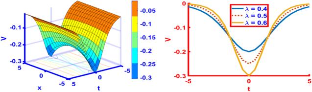
Figure 13. The 3D and 2D graphics for $s\left(t\right)=\,\tanh \left(\lambda {\rm{t}}\right)$ of the solution (68) with the particular values $l=5,$ $m=5,$ $n=2,$ $\delta =1,$ $\gamma =2,$ $\beta =1,$ $\alpha =3$ and $\lambda =0.4.$
Figure 14. The 3D and 2D graphics for $s\left(t\right)=\,\cos \left(\lambda {\rm{t}}\right)$ of the particular solution (75) with the particular values $l=4,$ $m=7,$ $n=2.5,$ $\alpha =3.5,$ $\beta =2.5,$ $\gamma =3.5,$ $\delta =8$ and $\lambda =0.6.$
Figure 15. The 3D and 2D graphics for $s\left(t\right)=\lambda {\rm{t}}$ of the particular solution (76) with the particular values $l=1,$ $m=7,$ $n=5,$ $\alpha =3,$ $\beta =0.5,$ $\gamma =1.5,$ $\delta =1$ and $\lambda =1.$
Figure 16. The 3D and 2 graphics for $s\left(t\right)=\,\cos (\lambda {\rm{t}})$ of the solution (77) with the parametric values $l=-0.9,$ $m=7,$ $n=2.5,$ $\alpha =3.5,$ $\beta =2.5,$ $\gamma =3.5,$ $\delta =8$ and $\lambda =0.1.$
Since $r\left(t\right)$ is an arbitrary function, without loss of generality we have considered $r\left(t\right)=\lambda {\rm{t}}.$ For the parametric values $h=2,\,k=1,\,\alpha =6,\,\beta =2,\,\gamma =2$ and $\lambda =2,$ the solution (24) demonstrate the periodic soliton and designated in figure 1. Periodic solitons perform a dynamic onward in characterizing the electrostatic wave potential in plasma physics. The space-time range for 3D graph is $-10\leqslant x,t\leqslant 10.$ Also, the two-dimensional plot with the time range $-15\leqslant t\leqslant 15$ is depicted for $\lambda =2,$ $2.1,$ $2.2$ which are identified by three different colors.
Figure 2 describes the periodic soliton nature represented by the solution (28). The suitable values of parameters with $r\left(t\right)=\lambda t$ are taken as $h=0.5,$ $k=0.2,$ $\alpha =0.3,$ $\beta =0.4,$ $\gamma =0.6$ and $\lambda =0.5$ for 3D and 2D graphs. The two-dimensional graph is portrayed at $\lambda =0.5,$ $0.506,$ $0.509$ with different colors. The space-time range of 3D and 2D graphs is $-5\leqslant x,t\leqslant 5.$
Also, the 3D graph in figure 3 reflects the bright solitonic nature for $r\left(t\right)=\,\sinh \left(\lambda t\right)$ of the solution (28) with the appropriate parametric values $h=0.7,$ $k=-1,$ $\alpha =-1,$ $\beta =2,$ $\gamma =3$ and $\lambda =0.2.$ The bright solitons are worthwhile to understand the behavior of charged carriers in quantum plasmas. The space-time range of 3D and 2D graphics is $-5\leqslant x,t\leqslant 5.$ The two-dimensional plot is drawn at $\lambda =0.2,$ $0.21,$ $0.22$ which are identified by diverse colors.
On the contrary, the solution (29) for the parametric values $h=4,$ $k=4,$ $\alpha =3,$ $\beta =-0.1,$ $\gamma =0.3$ and $\lambda =4$ represents pulse like singular periodic soliton, presented in figure 4 for $r\left(t\right)=\lambda t.$ The singular solitons are traveling wave solutions having discontinuities. The time-space range for 3D graph is $-5\leqslant x,t\leqslant 5,$ for 2D graph the time range is $-10\leqslant t\leqslant 10$ at $\lambda =4,$ $5,$ $6.$
Furthermore, the solution shapes in figure 5 show the compacton drawn from the solution (30) for $r\left(t\right)=\lambda {\rm{t}}$ with the particular values $h=2.8,$ $k=3,$ $\alpha =3,$ $\beta =2,$ $\gamma =1.9$ and $\lambda =2.$ Compactons are a sort of soliton with a dense support that can be used to describe ion-acoustic waves, electrostatics wave, quantum acoustic waves in plasma physics. The space-time range for 3D graph is $-5\leqslant x,t\leqslant 5.$ The two-dimensional plot is shown at $\lambda =2,$ $2.1,$ $2.2$ in different colors with the time range $-10\leqslant t\leqslant 10.$
Figure 6 indicates the periodic soliton for $r\left(t\right)=\lambda \,{\rm{t}}$ sketched from the solution (34) with the particular values $h=0.7,$ $k=1,$ $\alpha =0.4,$ $\beta =0.4,$ $\gamma =0.6$ and $\lambda =-1.$ The time-space range of 3D graph for real and imaginary parts of the solution (34) is $-10\leqslant x,t\leqslant 10.$
Figure 7, describes the bell-shape soliton portrayed from the solution (38) for $r\left(t\right)=\lambda {\rm{t}}$ with the parametric values $h=0.7,$ $k=1,$ $\alpha =0.4,$ $\beta =0.4,$ $\gamma =0.6$ and $\lambda =1.5.$ Bell-shaped solitons, which have infinite wings on both sides, are another sort of solitary wave solution useful signal management. The time-space range for 3D and 2D graph is $-5\leqslant x,t\leqslant 5.$ The two-dimensional plot is portrayed at $\lambda =1.5,$ $2,$ $2.5.$
The solution (40) exhibits the parabolic soliton for the values of $h=9,$ $k=-0.8,$ $\alpha =2,$ $\beta =4,$ $\gamma =6$ and $\lambda =-0.1$ with $r\left(t\right)=\lambda {\rm{t}}$ sketched in figure 8. The space-time range of 3D and 2D graph is $-5\leqslant x,t\leqslant 5.$ The two-dimensional plot is depicted at $\lambda =-0.1.$
The 3D graph in figure 9 shows the soliton nature for $s\left(t\right)=\,\sin \left(\lambda t\right)$ of the particular solution (63) with the suitable parametric values $l=-0.1,$ $m=0.3,$ $n=1,$ $\delta =0.8,$ $\gamma =0.6,$ $\beta =0.9,$ $\alpha =0.4$ and $\lambda =0.2.$ The space-time range of 3D graph for real and imaginary parts of the solution (63) is $-10\leqslant x,t\leqslant 10.$
On the other hand, figure 10 reflects the periodic soliton nature for $s\left(t\right)=\,\sin \left(\lambda {\rm{t}}\right)$ of the particular solution (66) with the particular values $l=0.6,$ $m=0.8,$ $n=1,$ $\alpha =2,$ $\beta =4,$ $\gamma =2,$ $\delta =1$ and $\lambda =1.$ The space-time range of 3D and 2D graph is $-8\leqslant x,t\leqslant 8.$ Also, the 2D graph is depicted at $\lambda =1,$ $1.2,$ $1.4$ which are specified by different colors.
Furthermore, the solution shapes in figure 11 is the bright-like soliton profile is interpreted from the solution (66) for $s\left(t\right)={{\rm{e}}}^{\lambda {\rm{t}}}$ with the suitable parametric values $l=5,$ $m=0.5,$ $n=2,$ $\alpha =3,$ $\beta =1,$ $\gamma =2,$ $\delta =2$ and, $\lambda =-0.4.$ This solution is descend from left to right asymptotic state. The space-time range for 3D and 2D graph is $-5\leqslant x,t\leqslant 5.$ Also, the two-dimensional plot is illustrated at $\lambda =-0.4,$ $-0.5,$ $-0.6.$
Figure 12 is the singular soliton characterized by the solution (67). The appropriate values of parameters with $s\left(t\right)=\,\sin (\lambda t)$ are taken as $l=1,$ $m=0.2,$ $n=0.9,$ $\delta =1,$ $\gamma =1.5,$ $\beta =2.5,$ $\alpha =1.5$ and $\lambda =0.1$ for 3D and 2D graphs. The two-dimensional graph is portrayed at $\lambda =0.1,$ $0.2,$ $0.3$ with different colors. The space-time range of 3D and 2D graphs is $-5\leqslant x,t\leqslant 5.$
Figure 13 represents the soliton like solution for $s\left(t\right)=\,\tanh (\lambda t)$ of the solution (68) with suitable parametric values $l=5,$ $m=5,$ $n=2,$ $\delta =1,$ $\gamma =2,$ $\beta =1,$ $\alpha =3$ and $\lambda =0.4.$ The space-time range for 3D and 2D graphs is $-5\leqslant x,t\leqslant 5.$ The two-dimensional plot is drawn at $\lambda =0.4,$ $0.5,$ $0.6$ which are specified by different colors.
Figure 14, is periodic soliton depicted from the solution (75) for $s\left(t\right)=\,\cos (\lambda {\rm{t}})$ with the suitable parametric values $l=4,$ $m=7,$ $n=2.5,$ $\alpha =3.5,$ $\beta =2.5,$ $\gamma =3.5,$ $\delta =8$ and $\lambda =0.6.$ The space-time range for 3D and 2D graph is $-5\leqslant x,t\leqslant 5.$ The two-dimensional plot is shown at $\lambda =0.6,$ $0.7,$ $0.8$ with different colors.
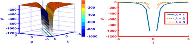
Figure 15 signifies the singular soliton for $s\left(t\right)=\lambda {\rm{t}}$ constructed from the solution (76) with the particular values $l=1,$ $m=7,$ $n=5,$ $\alpha =3,$ $\beta =0.5,$ $\gamma =1.5,$ $\delta =1$ and $\lambda =1.$ The time- space range of 3D and 2D graph is $-5\leqslant x,t\leqslant 5.$ Also, the two-dimensional plot is depicted at $\lambda =1,$ $2,$ $3$ which is shown in different colors.
The solution shape in figure 16 shows the plane soliton which is drawn from the solution (77) for $s\left(t\right)=\,\cos (\lambda {\rm{t}})$ with the parametric values $l=-0.9,$ $m=7,$ $n=2.5,$ $\alpha =3.5,$ $\beta =2.5,$ $\gamma =3.5,$ $\delta =8$ and $\lambda =0.1.$ The space time range for 3D and 2D graph is $-5\leqslant x,t\leqslant 5.$ Also, the two-dimensional plot is drawn at λ = 0.1, $0.2,$ $0.3$ which are identified by three different colors.
For simplicity, some graphical representations of the achieved solutions are not reported here. Figures 1–16 indicate the periodic, bright, singular periodic, bell-shaped, compacton, parabolic, plane-shaped solitons etc describe the physical behavior of instances modulated by extended QZK equation and (3 + 1)-dimensional ZK equation.
5. Conclusion
In this study, we have effectively contrived the enhanced MSE technique to search for standard, definitive, and large-scale soliton solutions of the new extended QZK and (3 + 1)-dimensional ZK equations. The solutions are revealed in rational function, trigonometric function, hyperbolic function, exponential function and their integration. Bright solitons, periodic solitons, compacton, bell-shaped, parabolic, singular periodic solitons, plane shaped solitons, and some distinct and general solitons have been established. The soliton solutions that are similar to the preceding solutions validate this study, and the generic soliton solutions will enrich the literature and be valuable in future research. Two and three-dimensional graphs of these solutions are portrayed to help understand physical phenomena, namely ion-acoustic waves, dense quantum plasma, electron thermal energies, ion plasmas, quantum acoustic waves, quantum Langmuir waves, etc. This study confirms that the enhanced MSE technique is an effective and useful mathematical tool and is applicable to other NLEEs in physics, engineering and mathematical physics.
The authors would like to express their gratitude to the anonymous referees for their insightful remarks and ideas to improve the quality of the article.
LuDSeadawyA RWangJArshadMFarooqU2019 Soliton solutions of the generalized third-order nonlinear Schrödinger equation by two mathematical methods and their stability Pramana93 1 9
KayumM AAkbarM AOsmanM S2020 Competent closed form soliton solutions to the nonlinear transmission and the low-pass electrical transmission lines Eur. Phys. J. Plus135 1 20
RezazadehHKorkmazAEslamiMMirhosseini-AlizaminiS M2019 A large family of optical solutions to Kundu-Eckhaus model by a new auxiliary equation method Opt. Quantum Electron.51 1 12
BaskonusH MKoçD ABulutH2016 New travelling wave prototypes to the nonlinear Zakharov-Kuznetsov equation with power law nonlinearity Nonlinear Sci. Lett. A7 67 76
8
TchierFAliyuA IYusufAIncM2017 Dynamics of solitons to the ill-posed Boussinesq equation Eur. Phys. J. Plus132 1 9
IncMAliyuA IYusufA2017 Dark optical, singular solitons and conservation laws to the nonlinear Schrödinger's equation with spatio-temporal dispersion Mod. Phys. Lett. B31 1750163
Al QurashiM MYusufAAliyuA IIncM2017 Optical and other solitons for the fourth-order dispersive nonlinear Schrödinger equation with dual-power law nonlinearity Superlattices Microstruct.105 183 197
KayumM AAraSOsmanM SAkbarM AGepreelK A2021 Onset of the broad-ranging general stable soliton solutions of nonlinear equations in physics and gas dynamics Results Phys.20 103762
OsmanM S2019 One-soliton shaping and inelastic collision between double solitons in the fifth-order variable-coefficient Sawada-Kotera equation Nonlinear Dyn.96 1491 1496
KumarSJiwariRMittalR CAwrejcewiczJ2021 Dark and bright soliton solutions and computational modeling of nonlinear regularized long wave model Nonlinear Dyn.104 661 682
18
KhanY2021 A novel type of soliton solutions for the Fokas-Lenells equation arising in the application of optical fibers Mod. Phys. Lett. B35 2150058
ZayedE MAlngarM E2021 Optical soliton solutions for the generalized Kudryashov equation of propagation pulse in optical fiber with power nonlinearities by three integration algorithms Math. Met. Appl. Sci.44 315 324
GepreelK AZayedE M EAlngarM E M2021 New optical solitons perturbation in the birefringent fibers for the CGL equation with Kerr law nonlinearity using two integral schemes methods Optik227 166099
KhanKAkbarM A2013 Application of exp-expansion method to find the exact solutions of modified Benjamin-Bona-Mahony equation World Appl. Sci. J.24 1373 1377
26
Ali AkbarMAliN H M2017 The improved F-expansion method with Riccati equation and its applications in mathematical physics Cogent Math.4 1282577
AkbarM AKayumM AOsmanM SAbdel-AtyA HEleuchH2021 Analysis of voltage and current flow of electrical transmission lines through mZK equation Results Phys.20 103696
KayumM AAraSBarmanH KAkbarM A2020 Soliton solutions to voltage analysis in nonlinear electrical transmission lines and electric signals in telegraph lines Results Phys.18 103269
KayumM ABarmanH KAkbarM A2021 Exact soliton solutions to the nano-bioscience and biophysics equations through the modified simple equation method Proc. of the 6th Int. Conf. on Mathematics and Computing Singapore Springer 469 482
30
KayumM ASeadawyA RAkbarA MSugatiT G2020 Stable solutions to the nonlinear RLC transmission line equation and the Sinh-Poisson equation arising in mathematical physics Open Phys.18 710 725
AslanE CTchierFIncM2017 On optical solitons of the Schrödinger-Hirota equation with power law nonlinearity in optical fibers Superlattices Microstruct.105 48 55
KayumM ARoyRAkbarM AOsmanM S2021 Study of W-shaped, V-shaped, and other type of surfaces of the ZK-BBM and GZD-BBM equations Opt. Quantum Electron.53 387
AlmusawaHNur AlamMFayz-Al-AsadMOsmanM S2021 New soliton configurations for two different models related to the nonlinear Schrödinger equation through a graded-index waveguide AIP Adv.11 065320
LiuJ GOsmanM SWazwazA M2019 A variety of nonautonomous complex wave solutions for the (2 + 1)-dimensional nonlinear Schrödinger equation with variable coefficients in nonlinear optical fibers Optik180 917 923
DingYOsmanM SWazwazA M2019 Abundant complex wave solutions for the nonautonomous Fokas–Lenells equation in presence of perturbation terms Optik181 503 513
MoslemW MAliSShuklaP KTangX YRowlandsG2007 Solitary, explosive, and periodic solutions of the quantum Zakharov-Kuznetsov equation and its transverse instability Phys. Plasmas14 082308
BaskonusH MBulutHSulaimanT A2017 Investigation of various travelling wave solutions to the extended (2 + 1)-dimensional quantum ZK equation Eur. Phys. J. Plus132 1 8
BhrawyA HAbdelkawyM AKumarSJohnsonSBiswasA2013 Solitons and other solutions to quantum Zakharov-Kuznetsov equation in quantum magneto-plasmas Indian J. Phys.87 455 463
ZayedE M EAlurrfiK A E2016 Extended generalized (G′/G) -expansion method for solving the nonlinear quantum Zakharov-Kuznetsov equation Ric. di Mat.65 235 254
LuDSeadawyA RArshadMWangJ2017 New solitary wave solutions of (3 + 1)-dimensional nonlinear extended Zakharov-Kuznetsov and modified KdV-Zakharov-Kuznetsov equations and their applications Results Phys.7 899 909
ZayedE MShahootA MAlurrfiK A2018 The (G′/G,1/G) -expansion method and its applications for constructing many new exact solutions of the higher-order nonlinear Schrödinger equation and the quantum Zakharov-Kuznetsov equation Opt. Quantum Electron.50 96
RoshidM MAliM ZRezazadehH2020 Kinky periodic pulse and interaction of bell wave with kink pulse wave propagation in nerve fibers and wall motion in liquid crystals Partial Differ. Equ. Appl. Math.2 100012
ZhangCZhangZ2017 Application of the enhanced modified simple equation method for Burger-Fisher and modified Volterra equations Adv. Differ. Equ.2017 1 8
IslamM SRoshidM MRahmanA LAkbarM A2019 Solitary wave solutions in plasma physics and acoustic gravity waves of some nonlinear evolution equations through enhanced MSE method J. Phys. Commun.3 125011


