Entropy generation is one of the key features in analysis as it exhibits irreversibility of the system. Therefore, the present study investigates the entropy generation rate in a mixed convective peristaltic motion of a reactive nanofluid through an asymmetrical divergent channel with heat and mass transfer characteristics. The endorsed nanofluid model holds thermophoresis and Brownian diffusions. Mathematical modeling is configured under the effects of mixed convection, heat generation/absorption and viscous dissipation. A chemical reaction is also introduced for the description of mass transportation. The resulting system of differential equations is numerically tackled by employing the Shooting method. The findings reveal that entropy generation rises by improving the Brownian motion and thermophoresis parameters. The temperature of the nanofluid decreases due to rising buoyancy forces caused by the concentration gradient. The concentration profile increases by increasing the chemical reaction parameter. The velocity increases by enhancing the Brownian motion parameter.
Y Akbar, F M Abbasi, U M Zahid, S A Shehzad. Effectiveness of heat and mass transfer on mixed convective peristaltic motion of nanofluid with irreversibility rate[J]. Communications in Theoretical Physics, 2021, 73(10): 105004. DOI: 10.1088/1572-9494/ac10bf
1. Introduction
The mechanism of nanofluids is becoming a hot topic for research owing to their heat conductive properties. Typically, a nanofluid is a dilute aggregation of fibers and particles of nanometer scale distributed in a carrier liquid. Nanomaterials are composed of metals, their oxides and nanotubes, whereas base liquids include engine oils, lubricants, grease, water and ethylene glycol etc. Some nanofluids possess idiosyncratic properties. They have had a broad array of applications in many biomedical, industrial and engineering systems. Some of them include domestic refrigerators, fission and fusion reactions, fuel cells, cancer treatments, chemotherapy, hybrid-powered engines, milk sterilization, and electronic cooling systems. In 1995, innovative ideas of nanofluids were reported by Choi [1]. Later, Buongiorno [2] stated that nanofluids are the colloidal suspensions of small particles in liquids. In this study, the author also designed a model to assess the flow of nanoliquids using Brownian motion and thermophoresis effects. Prasad et al [3] reported a new concept to deliver nanomedicines. The main aim of this research was to treat rheumatoid arthritis. Kleinstreuer and Feng [4] conducted an experimental and theoretical study on optimizing nanofluids' thermal conductivity. A water-based nanoliquid moving over wavy surfaces in a porous space of spherical packing beds was highlighted by Hassan et al [5]. Vallejo et al [6] studied Ag–graphene-based hybrid nanoliquids for direct solar absorption. Recently, Shahrestani et al [7] numerically reviewed the fluid flow and thermal analysis of ${\mathrm{Al}}_{2}{{\rm{O}}}_{3}/{{\rm{H}}}_{2}{\rm{O}}$ nanoliquid inside a microchannel of inner diameter 0.1 mm.
Peristalsis is a fluid flow mechanism that occurs due to the successive series of muscle relaxation and contraction by which fluids are transferred from one place to another in a physiological system. Peristaltic flows are encountered in cilia motion, movement of spermatozoa, heart–lung and dialysis machines, medical infusion pumps and in rocket chamber fuel control technologies. In 1966, Latham [8] proposed a mechanism of liquid motion via peristaltic pump. Shapiro et al [9] made a considerable development on the mathematical modeling of peristaltic motion [8] and explored this mechanism by applying ‘long wavelength and small Reynolds number assumptions.' This research employed both theoretical and numerical methods. Akbar and Nadeem [10] discussed the peristaltic movement of a nanoliquid with endoscopic effects. The process of peristalsis has been studied by many researchers both theoretically and experimentally [11–19]. Riaz et al [20] explored the peristaltic propulsion of a Jeffrey nanoliquid through a porous rectangular duct.
The aspects of Brownian motion and thermophoresis are very important in the fields of science and technology. These effects are of great importance in the production of germanium oxide and silicon, etc. Beg and Tripathi [21] presented a theoretical analysis to explore the phenomenon of peristalsis with double-diffusive convection in nanoliquids via a deformable channel. For this review, the authors utilized Buongiorno's model to investigate the behavior of a nanoliquid. Peristaltic transportation of a magnetohydrodynamic (MHD) nanoliquid under the influence of Brownian motion and thermophoresis were highlighted by Hayat et al [22]. A numerical study on peristaltic motion of nanoliquids between the gap of two coaxial tubes with distinct structures and configurations was conducted by Ellahi et al [23]. Khan et al [24] analyzed the movement of non-Newtonian material subject to Dufour and Soret impacts over a porous space. The effects of wall flexibility with convective conditions on MHD peristaltic motion of an Eyring–Powell nanoliquid were highlighted by Nisar et al [25].
In thermal design and heat transfer, the analysis of the second law of thermodynamics is a widely used and useful tool. The study of entropy production is indeed one of the main aspects in analysis because it illustrates the disorder of the system. When any engineering system operates, it encounters irreversible energy losses that affect the efficiency of the machine. Therefore, circumstances are needed that minimize the production of entropy. The innovative idea of entropy generation (second law) was explained by Bejan [26]. In this analysis, the author outlined the key ways to minimize entropy at the system level of the structure. Nadeem and Sadia [27] studied entropy generation for a Johnson–Segalman fluid by assuming variable viscosity. Akbar et al [28] studied entropy generation for peristalsis of $\mathrm{Cu}+{{\rm{H}}}_{2}{\rm{O}}$ nanoliquid. Abbas et al [29] studied irreversible analysis for peristaltic movement of nanoliquids flowing in a two-dimensional (2D) channel with compliant walls. Farooq et al [30] explored the role of entropy production in peristalsis of multi- and single-walled carbon nanotubes. Consideration of entropy production for peristaltic transportation of $\mathrm{Cu}-{{\rm{H}}}_{2}{\rm{O}}$ nanoliquid with radiative heat flux was provided by Akbar et al [31]. MHD peristaltic transportation of a Sutterby nanoliquid with Hall current and mixed convection was highlighted by Hayat et al [32]. Some important studies related to irreversibility analysis for peristaltic transport of a nanoliquid can also be viewed in references [33–39].
In view of these investigations, the main aim of the present study is to address the irreversibility rate, heat and mass transfer for peristaltic flow of a reactive nanofluid flowing through a divergent channel. The effects of thermophoresis, chemical reaction and Brownian motion are taken into consideration. Lubrication theory is used in the mathematical formulation. The Shooting method is employed to obtain the solution of differential equations. Entropy generation, Bejan number, mass and heat transfers, and skin friction are addressed under the influence of different pertinent parameters. Further, comparisons of heat, mass transfer rate and skin friction at the channel wall in light of two different numeric methods are also provided. The present study finds its application in transport phenomena in chemical engineering and energy systems to increase the heat capacity of machines.
2. Problem formulation
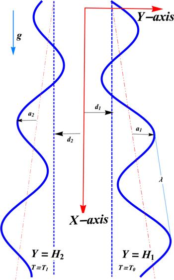
A 2D mixed convective peristaltic motion of reactive nanofluid through a divergent channel is considered. The wave trains are propagating with velocity c on the channel walls. Further, the channel is assumed to be asymmetric. A physical model of the problem is shown in figure 1. Mathematically, deformation in the channel walls is defined as [16]:
where ${d}_{1}+{d}_{2}$, a1, a2, c, t, m, γ and λ are the channel width, amplitudes, wave speed, time, nonuniform parameter, phase difference and wavelength, respectively. The governing equations for the present model using chemical reaction, thermophoresis, mixed convection, viscous dissipation and Brownian motion are given as [24, 33, 38]:
In the above equations P, Cf, $\hat{{\gamma }_{c}}$, DB, DT, C, α and ${\alpha }^{* }$ represent pressure, specific heat of fluid, chemical reaction rate, mass diffusivity, thermal diffusion, concentration, and thermal and concentration expansion coefficients, respectively.
Here ψ, Gt, Br, Gc, Sc, Nb, ${\gamma }_{c}$, Nt, and Pr are the dimensionless stream function, temperature Grashof number, Brinkman number, concentration Grashof number, Schmidt number, Brownian motion parameter, chemical reaction parameter, thermophoresis parameter and Prandtl number, respectively. Determining the nondimensional flow rates η and F, defined by [16]:
The Bejan number $({B}_{e})$ is the ratio of entropy produced by conduction to the total entropy. The mathematical interpretation of the Bejan number $({B}_{e})$ is expressed as follows [33]:
For numerical solution we intend to use the Shooting technique with RK-4 on differential equations (9)–(12) subject to boundary conditions (14). In this connection the boundary conditions (14) for the system of differential equations (9)–(12) are simplified into initial conditions. Therefore, the prescribed problem to be addressed is as follows:
Hence, the stated problem is converted into four systems of equations. These equations are further simplified to a system of first-order differential equations. The system of differential equations are then solved numerically by using the Shooting technique with the RK-4 method. Appropriate values of unknown initial conditions ${\xi }_{1}$, ${\xi }_{2}$, ${\xi }_{3}$ and ${\xi }_{4}$ are approximated and optimized through Newton's technique until the boundary conditions are met. The step scale is considered as ${\rm{\Delta }}h=0.05$ and convergence criterion is taken as 10−6. All necessary calculations are performed in Mathematica software.
5. Results and discussion
This section provides the graphs of different flow quantities for several parameters of interest. Plots for heat transfer, irreversible rate, mass transfer and velocity profile are presented and analyzed.
5.1. Heat transfer analysis
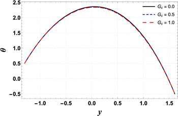
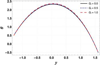
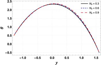
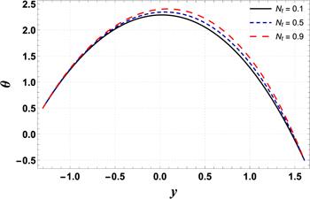
Analysis of temperature profile is presented through figures 2–5. The maximum value of temperature profile is observed near the center of the channel. Figure 2 indicates that the temperature profile decreases by increasing buoyancy forces caused by concentration difference (Gc). The displayed result is due to an increment in viscosity which leads to a drop in temperature. However, figure 3 shows that temperature increases by improving the temperature Grashof number (Gt). Physically, it refers to the condition where improved buoyancy forces are strengthened due to the temperature gradient. Figure 4 shows that temperature increases for a rise in Nb. The reason is that kinetic energy is augmented as Nb is improved which incorporates it into internal energy and thus raises the temperature within the channel. An increase in temperature is obtained by increasing the amount of the thermophoresis parameter (Nt) (see figure 5). For higher Nt, nanoparticles migrate from warm regions to cool regions and hence the temperature increases. Here, the numerical outcomes presented via figures 4 and 5 are found to be well matched with the results reported by Hayat et al [32] and Ellahi et al [23].
Numerical values of the heat transfer rate at the channel wall ($-\theta ^{\prime} ({h}_{1})$) for variations in Gt, Gc, Nt, and Nb are shown in table 1. It is seen that ($-\theta ^{\prime} ({h}_{1})$) increases when Gt is assigned higher values. This fact shows that mixed convection improves heat transfer phenomena between the solid boundary and the base fluid. A similar trend is also seen for Nb and Nt. However, ($-\theta ^{\prime} ({h}_{1})$) decreases for large Gc. Moreover, it is interesting to note that results calculated by both methods, i.e. the Shooting method and NDSolve, are in good agreement.
Table 1. Comparison of $-\theta ^{\prime} ({h}_{1})$ by using the Shooting method and the built-in function NDSolve in Mathematica.
Gt
Gc
Nt
Nb
Shooting method
NDSolve
Difference
0.5
4.058 59
4.0586
0.000 01
1.0
4.065 21
4.065 22
0.000 01
1.5
4.084 88
4.084 89
0.000 01
0.0
4.0851
4.085 11
0.000 01
0.5
4.058 59
4.0586
0.000 01
1.0
4.037 63
4.037 64
0.000 01
0.2
3.819 07
3.819 08
0.000 01
0.4
3.976 66
3.976 67
0.000 01
0.6
4.142 69
4.142 71
0.000 02
0.2
3.930 51
3.930 52
0.000 01
0.4
4.016 46
4.016 47
0.000 01
0.6
4.100 28
4.1003
0.000 02
5.2. Entropy generation
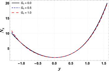
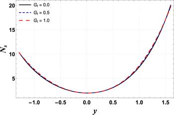
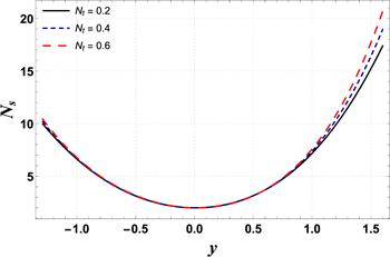
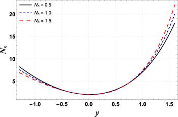
Figures 6–9 demonstrate the change in entropy generation (Ns) for different values of Gc, Gt, Nt and Nb. Figure 6 shows that through enhancing the values of Gc, entropy generation decreases. This is mainly due to a rise in buoyancy forces caused by the concentration difference, which lowers the temperature and contributes to a decrease in entropy generation. However, figure 7 indicates that entropy generation is enhanced by increasing the values of Gt. This occurs due to mixed convection caused by temperature differences, as mixed convection helps the nanoliquid in achieving higher temperatures, resulting in increased entropy production. It is visualized in figures 8 and 9 that increases in Nt and Nb enhance entropy generation. This is because kinetic energy increases with increases in Nt and Nb, which generates heat in the system, resulting in increased irreversibility in the system.
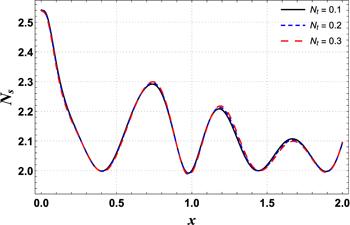
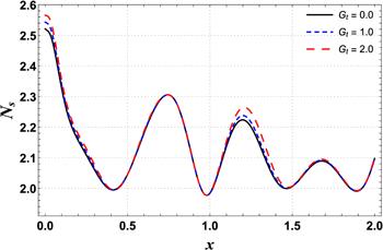
Figures 10 and 11 are outlined to show the effects of Nt and Gt on entropy generation along the channel's length. These graphs show oscillating behavior with the highest value near a wider portion of the channel. Figure 10 shows that entropy increases by improving Nt. A similar trend is seen for Gt (see figure 11). By improving buoyancy forces, the randomness in a system rises and hence the irreversibility rate increases.
Figure 11. Effects of Gt on Ns versus axial distance.
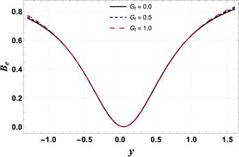
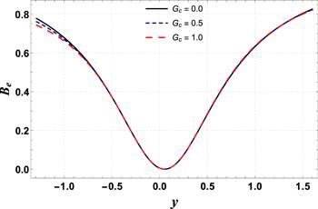
Figures 12 and 13 provide the distribution of Bejan number $({B}_{e})$ for different values of Gt and Gc. These graphs show that the Bejan number reaches its minimum value near the center of the channel, while the maximum value appears near the channel walls. The Bejan number has an increasing effect by increasing the values of Gt (see figure 12). This is due to an increase in heat transfer irreversibility over total irreversibility. However, the Bejan number has a decreasing behavior for enhanced values of Gc (see figure 13).
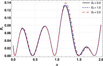
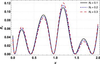
Figures 14 and 15 are outlined to show the effects of Nt and Gt on the Bejan number along the channel's length. These plots exhibit sinusoidal behavior with the highest value near the wider portion of the channel. Figure 14 shows that the Bejan number increases by increasing Gt. A similar trend is also seen for Nt (see figure 15).
Figure 15. Effects of Gt on Be versus axial distance.
5.3. Mass transfer analysis
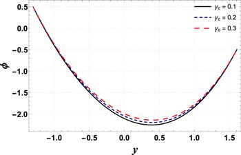
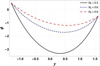
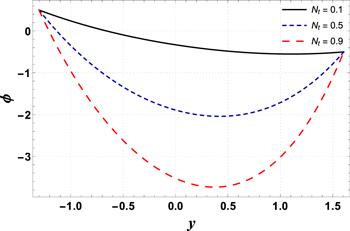
Figures 16–19 display the consequences of Sc, ${\gamma }_{c}$, Nb, and Nt on concentration profile $(\phi )$. Figure 16 indicates that φ increases when Sc is increased. This is primarily due to an increase in momentum diffusivity. A similar trend is noted for ${\gamma }_{c}$ (see figure 17). The concentration increases when ${\gamma }_{c}$ is assigned higher values. As the chemical reaction enhances the interfacial mass transfer rate, thus the local concentration decreases, resulting in an increased concentration flux. It is inferred from figures 18 and 19 that φ increases with an enhancement in Nb and decreases for larger Nt. When Nt increases, there is a decrease in viscosity which leads to a decrease in φ.
Table 2 shows the effects of Sc, ${\gamma }_{c}$, Nt and Nb on mass transfer rate at the channel wall ($\phi ^{\prime} ({h}_{1})$). Table 2 shows that ‘$\phi ^{\prime} ({h}_{1})$' augments by increasing the values of Nt while it decreases by increasing Sc, ${\gamma }_{c}$ and Nb. Moreover, it is interesting to note that the results calculated by both methods are in good agreement.
Table 2. Comparison of $\phi ^{\prime} ({h}_{1})$ by using the Shooting method and the built-in function NDSolve in Mathematica.
Sc
${\gamma }_{c}$
Nt
Nb
Shooting method
NDSolve
Difference
0.2
2.923 02
2.92303
0.000 01
0.4
2.751 89
2.75188
0.000 01
0.6
2.611 37
2.61138
0.000 01
0.1
3.115 39
3.11540
0.000 01
0.2
3.091 71
3.09172
0.000 01
0.3
3.068 67
3.06868
0.000 01
0.2
0.843 57
0.84358
0.000 01
0.4
2.197 92
2.19793
0.000 01
0.6
3.681 78
3.68179
0.000 01
0.2
7.593 69
7.59370
0.000 01
0.4
3.701 53
3.70154
0.000 01
0.6
2.403 82
2.40383
0.000 01
5.4. Flow behavior analysis
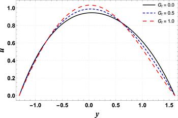
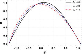
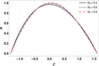
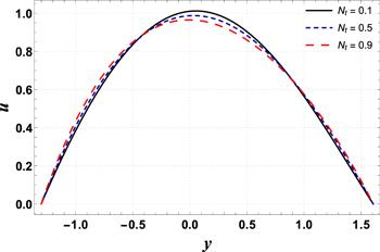
Figures 20–23 are designed to compute the variations in Gt, Gc, Nb and Nt on velocity profile. These plots show that an extreme value of velocity occurs near the channel center. From figure 20 it is noted that velocity is an increasing function of Gt. This is because an increase in Gr leads to a decrease in viscosity. This activity causes less resistance to flow and therefore increases velocity. In contrast to the previous case, velocity decreases with an increase in Gc (see figure 21). This is because Gc with its increasing values improves the concentration of the nanofluid and results in a decrease in velocity. Figure 22 shows an increase in velocity as Nb is enhanced. It is found that Nb lowers the viscosity of the fluid due to its heat absorbing properties and thus tends to increase the fluid velocity. A decreasing effect on velocity is reported for increasing Nt as it makes the nanofluid denser (see figure 23).
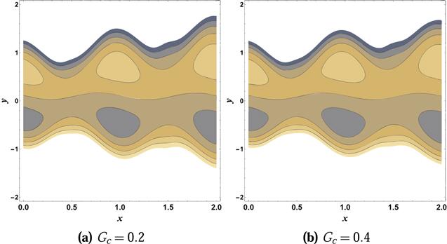
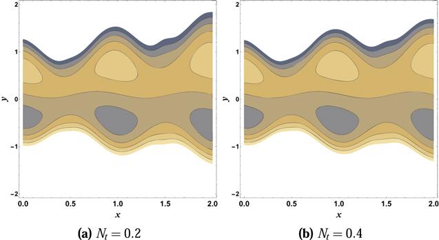
It is important to look at the nature of streamlines under the influence of various parameters that affect the flow characteristics. The most important characteristic of peristaltic flow is associated with the circulation of streamline, characterized as trapping that leads to the formation of the trapped volume of liquids, which is called a bolus. This captured bolus is carried along peristaltic waves. This tendency is extremely beneficial for transporting fluids through the body in a proper manner. This phenomenon is examined through figures 24 and 25. From these plots, it is noted that the bolus formation and streamline pattern slightly changes by enhancing Gc and Nt.
Table 3 displays the numerical results of Gt, Gc, Nb and Nt on skin friction at the wall. Table 3 shows that skin friction at the wall consistently augments with an increase in Gt and Nt whereas it reduces with Gc and Nb.
Table 3. Comparison of skin friction by using the Shooting method and the built-in function NDSolve in Mathematica.
Gt
Gc
Nt
Nb
Shooting method
NDSolve
Difference
0.5
−1.06618
−1.06617
0.000 01
1.0
−0.73846
−0.73845
0.000 01
1.5
−0.40594
−0.40593
0.000 01
0.0
−1.01375
−1.01374
0.000 01
0.5
−1.06618
−1.06617
0.000 01
1.0
−1.11807
−1.11806
0.000 01
0.2
−0.96284
−0.96283
0.000 01
0.4
−1.03219
−1.03218
0.000 01
0.6
−1.09966
−1.09968
0.000 01
0.2
−1.32612
−1.32611
0.000 01
0.4
−1.10898
−1.10897
0.000 01
0.6
−1.03813
−1.03812
0.000 01
6. Conclusions
Entropy generation rate, heat and mass transfer analysis for mixed convective peristaltic transportation of a reactive nanofluid under the effects of thermophoresis and Brownian motion are investigated. The major findings produced from the present study are:
•
The temperature of a nanofluid increases by increasing the Brownian motion parameter.
•
Entropy generation enhances by improving the Brownian motion parameter.
•
An increase in the thermophoresis parameter produces more entropy.
•
The Bejan number has an increasing effect for increasing temperature Grashof number.
•
Concentration of nanoparticles improves when the Brownian motion parameter is increased, and decreases by enhancing the thermophoresis parameter.
•
An increase in the chemical reaction parameter improves the concentration characteristics of nanoparticles.
•
The mass transfer rate at the wall enhances by increasing the thermophoresis parameter. On the other hand, it decreases by enhancing the Schmidt number and chemical reaction parameter.
•
An augmentation in axial velocity is seen for a large temperature Grashof number while it decreases by increasing the concentration Grashof number.
•
Velocity increases by enhancing the Brownian motion parameter while it decreases for a large thermophoresis parameter.
ChoiS UEastmanJ A1995Enhancing Thermal Conductivity of Fluids with Nanoparticles (No. ANL/MSD/CP-84938; CONF-951135-29) Lemont, IL Argonne National Lab
2
BuongiornoJ2006Convective Transport in Nanofluids128 240 250
Irandoost ShahrestaniMMalekiASafdari ShadlooMTliliI2020 Numerical investigation of forced convective heat transfer and performance evaluation criterion of ${\mathrm{Al}}_{2}{{\rm{O}}}_{3}/\mathrm{water}$ nanofluid flow inside an axisymmetric microchannel Symmetry12 120
MakindeO DReddyM GReddyK V2017 Effects of thermal radiation on MHD peristaltic motion of Walters-B fluid with heat source and slip conditions J. Appl. Fluid Mech.10 1105 1112
ReddyK VMakindeO DReddyM G2018 Thermal analysis of MHD electro-osmotic peristaltic pumping of Casson fluid through a rotating asymmetric micro-channel Indian J. Phys.92 1439 1448
KothandapaniMPrakashJ2015 Effects of thermal radiation parameter and magnetic field on the peristaltic motion of Williamson nanofluids in a tapered asymmetric channel International J. Heat Mass Transfer81 234 245
MekheimerK SHasonaW MAbo-ElkhairR EZaherA Z2018 Peristaltic blood flow with gold nanoparticles as a third grade nanofluid in catheter: applications of cancer therapy Phys. Lett. A382 85 93
ZeeshanABhattiM MMuhammadTZhangL2020 Magnetized peristaltic particle–fluid propulsion with Hall and ion slip effects through a permeable channel Physica A550 123999
RiazAZeeshanABhattiM MEllahiR2020 Peristaltic propulsion of Jeffrey nano-liquid and heat transfer through a symmetrical duct with moving walls in a porous medium Physica A545 123788
BegO ATripathiD2011 Mathematica simulation of peristaltic pumping with double-diffusive convection in nanofluids: a bio-nano-engineering model Proc. Inst. Mech. Eng., Part N225 99 114
HayatTAbbasiF MAl-YamiMMonaquelS2014 Slip and Joule heating effects in mixed convection peristaltic transport of nanofluid with Soret and Dufour effects J. Mol. Liq.194 93 99
EllahiRZeeshanAHussainFAsadollahiA2019 Peristaltic blood flow of couple stress fluid suspended with nanoparticles under the influence of chemical reaction and activation energy Symmetry11 276
NadeemSSadiaH2013 Influence of temperature dependent viscosity and entropy generation on the flow of a Johnson–Segalman fluid Walailak J. Sci. Technol.10 553 579
28
AkramSZafarMNadeemS2018 Peristaltic transport of a Jeffrey fluid with double-diffusive convection in nanofluids in the presence of inclined magnetic field Int. J. Geom. Meth. Mod. Phys.15 1850181
FarooqSHayatTAlsaediAAsgharS2018 Mixed convection peristalsis of carbon nanotubes with thermal radiation and entropy generation J. Mol. Liq.250 451 467
AkbarYAbbasiF MShehzadS A2020 Thermal radiation and Hall effects in mixed convective peristaltic transport of nanofluid with entropy generation Appl. Nanoscience10 5421 5433
HayatTNisarZAlsaediAAhmadB2021 Analysis of activation energy and entropy generation in mixed convective peristaltic transport of Sutterby nanofluid J. Therm. Anal. Calorim.143 1867 1880
AkbarYAbbasiF MShehzadS A2020 Effectiveness of Hall current and ion slip on hydromagnetic biologically inspired flow of $\mathrm{Cu}-{\mathrm{Fe}}_{3}{{\rm{O}}}_{4}/{{\rm{H}}}_{2}{\rm{O}}$ hybrid nanomaterial Phys. Scr.96 025210
RiazABhattiM MEllahiRZeeshanAM SaitS2020 Mathematical analysis on an asymmetrical wavy motion of blood under the influence entropy generation with convective boundary conditions Symmetry12 102
AkbarYAbbasiF M Irreversibility analysis of nanofluid flow induced by peristaltic waves in the presence of concentration-dependent viscosity Heat Transfer 1 18


